
1. Introduction
The largest issues for offshore structures in terms of steels are the development of heavy thick plate and heavy wall thickness pipe, improvement of the corrosion resistance, and the development of high toughness steel at cryogenic temperatures. Improving the fatigue strength of welded joints is an important issue from the viewpoint of the design of offshore structures because the fatigue lives at weld joints can be reduced due to stress concentrations and weld imperfections.
Some S-N curves, also known as Wöhler curves, are necessary to evaluate the fatigue life of offshore structures. Because the formation of S-N curves for real structures has considerable limitations in terms of the size of the test equipment and the experimental budget, it is common to derive the S-N curve through experiments on small specimens instead of the actual structure.
Experiments on the stress ranges of at least three levels are required to produce a single S-N curve, but at least 10 levels or more are required for a reliable S-N curve. On the other hand, small sized-specimens may have different imperfections, such as residual stress and initial deformation, because of the different manufacturing processes. Even if a small specimen is taken from an actual structure, there are insufficient aspects to simulate real structures accurately due to the release of the residual stress.
When evaluating the fatigue life of an actual structure using the small specimen-based S-N curve, it is essential to recognize the stochastic characteristics of the S-N curve. The S-N curve, including a specified survival or failure probability, is defined as a basic design S-N curve.
The symbols and formulae describing a basic design S-N curve differ according to the fatigue guidelines, recommendations, or codes. Let the guideline, recommendation, and code associated with fatigue denote the fatigue codes. In this paper, the basic design S-N curves of a non-tubular member made of steel and the corresponding material constants by the fatigue codes were analyzed, and the S-N curves were compared according to the codes.
The fatigue codes provide the basic design S-N curves for each structural detail category (SDC). The SDC is also called the classification of details, detail category, classification reference, and joint classification. The SDC is determined by the type of stress, geometry detail, and the direction of stress relative to the potential fatigue crack (normal and shear stresses) (BSI, 2015).
The fatigue codes considered in this study were DNVGL-RP-C203 (DNV GL, 2016), Guide for Fatigue Assessment of Offshore Structures (ABS, 2003), BS 7608 (BSI, 2015), and IIW-1823 (IIW, 2008), and Eurocode3 (BSI, 2005). In this paper, these codes are termed as DNV GL, ABS, BS, Det Norske Veritas, and EC3, respectively.
2. Notations
In this review paper, five codes (DNV GL, ABS, BS, IIW, and EC3) were analyzed intensively. Table 1 lists the symbols used here.
Unless stated otherwise, the basic design S-N curves in the five codes are based on the nominal stress, and the different notations for the nominal stress are used for each code. Here, the nominal stress means stress that does not include any form of stress concentration. The extrapolated stress, including the stress concentration factor (SCF) caused by the geometric detail, is called hot-spot stress, and the corresponding notations are used for each code. The basic design S-N curve uses a stress range rather than a stress amplitude, and various stress range notations are shown for each code. Some codes (DNV GL, ABS, and BS) plot the S-N curves with slope and intercept, while others (IIW and EC3) use the fatigue strength (FAT) and slope at 2 million cycles.
To represent the survival probability applied to the basic design S-N curve, some codes (DNV GL, ABS, and BS) provide the standard deviation of the logarithmic life to failure. Therefore, a mean S-N curve is suggested together. In contrast, IIW and EC3 provide a basic design S-N curve by specifying the 95% survival probability instead of the standard deviation.
3. Types of Stresses
The stress range used for the S-N curve is very important. That is, nominal stress, hot-spot stress, and effective notch stress are used mainly in the S-N curve.
3.1 Nominal Stress
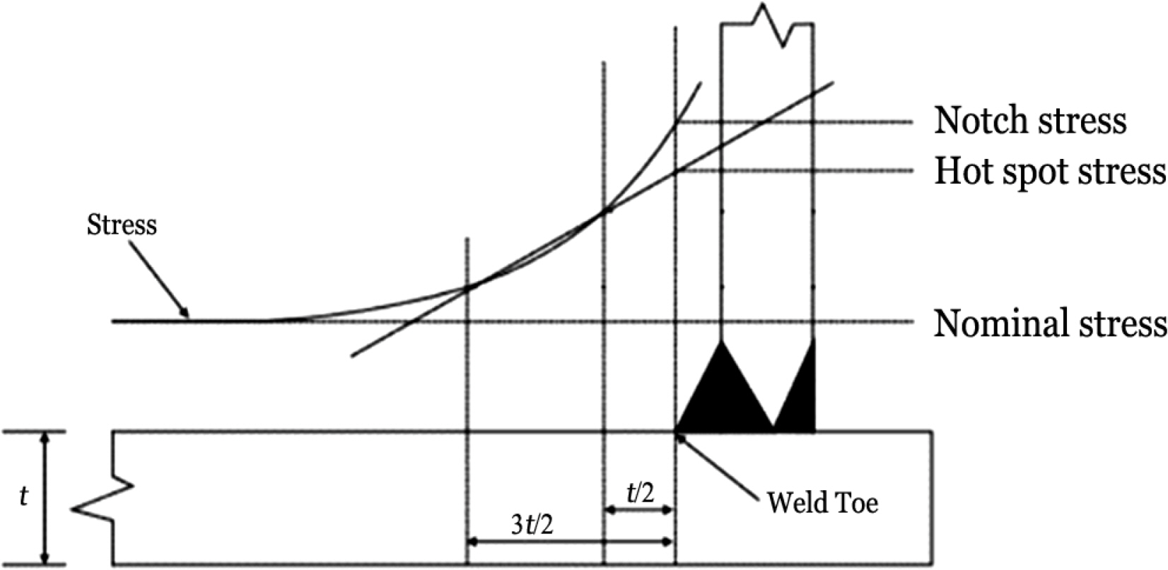
The nominal stress is the stress away from the local stress concentration area, where fatigue cracking can occur. That is, the nominal stress does not include welding residual stresses and SCFs due to the weld geometry. The stress concentration must not be included in the nominal stress (see Fig. 1). Most of the basic design S-N curves in the five codes are based on the nominal stress approach.
3.2 Effective Notch Stress
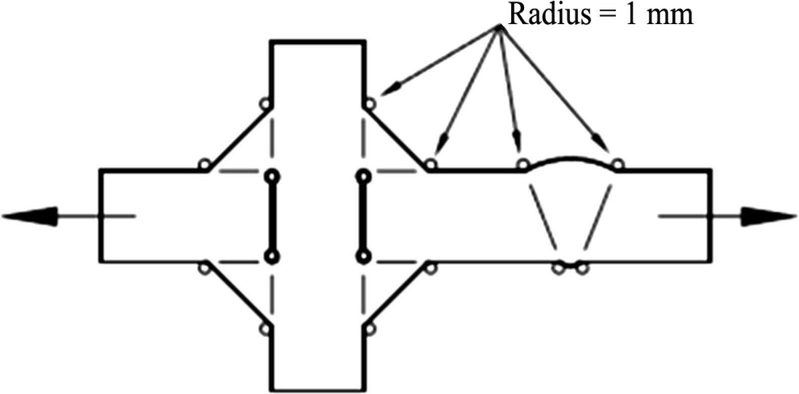
As shown in Fig. 2, the local stress at a weld toe, which is called the effective notch stress, was calculated by modeling the notch radius of 1 mm. Because the effective notch stress approach assumes a very small notch radius, it cannot be obtained through direct measurements and can only be derived through finite element analysis with a very fine mesh.
The effective notch stress approach is applicable to structures with thicknesses of 5 mm or more. Internal defects or surface roughness cannot be modeled as the effective notch radii. In addition, the effective notch stress approach cannot be applied to cases under the loads parallel to the weld or root gap. DNV GL and IIW support the basic design of S-N curves based on the effective notch stress approach.
3.3 Hot-spot Stress
The hot-spot stress is the imaginary stress obtained by extrapolating the surface stresses at the two or three points in front of the weld toe. The hot-spot stress approach is used mainly in the shipbuilding and offshore industries because it can derive the hot-spot stress at a low cost with a relatively coarser mesh. The hot-spot stress can be calculated by finite element analysis or measurements using strain gauges.
When applying finite element analysis, the hot-spot stresses can be calculated using either the shell or solid elements. When shell elements are used, there is no need to contain weld beads. It is common to include weld beads for solid elements application.
Weld residual stresses and stress concentrations due to the weld detail and structural geometry should not be included in the hot-spot stress. Alternatively, the SCFs for representative structural details can be obtained from handbooks or other codes.
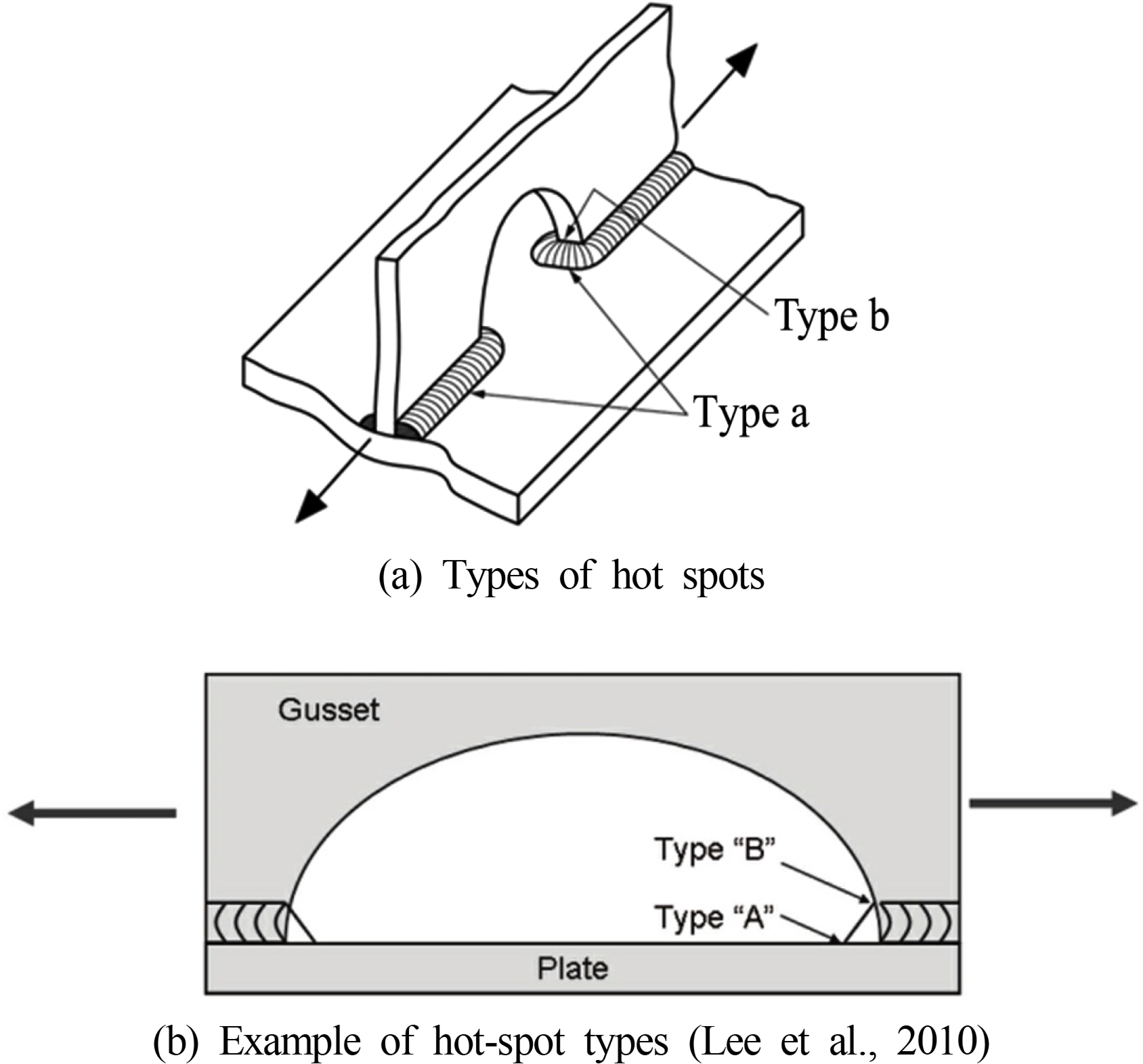
According to BS and IIW, the hot-spot stress is divided into types a and b. Type a is a case where the hot-spot stress is affected by the base plate thickness, while the base plate thickness varies the hot pot stress in the case of type b (see Fig. 3(a)). In Fig. 3(b), point A is classified as a type a hot spot because it is affected by the base plate thickness, and point B should be classified as a type b hot spot.
3.3.1 Type a hot-spot stress
The type a hot-spot stress is obtained by linearly extrapolating the stress either at 0.4t and 1.0t away or 0.5t and 1.5t away from the weld toe (see Eqs. (1) and (2)). This type of hot-spot stress can be determined by quadratic extrapolation of the stresses at 0.4t, 0.9t, and 1.4t away from the weld toe (see Eq. (3)). Here, t means the base plate thickness.
According to IIW, the hot-spot stresses should be obtained by the mesh sizes. That is, Eq. (1) or (3) should be applied for a fine mesh model that has an element size less than the base plate thickness, while Eq. (2) is used for a coarse mesh model with an element size equal to the base plate thickness.
3.3.2 Type b hot-spot stress
According to IIW, Eqs. (4) and (5) are applied to the fine and coarse mesh models, respectively. The subscripts in Eqs. (4) and (5) refer to the physical distance from the weld toe.
In the case of BS, there is no special indication or recommendation for the finite element sizes. Provided the surface stresses can be derived at the specified positions, Eqs. (4) and (5) can be applied to both fine and coarse mesh models.
Because DNV GL and ABS do not distinguish the hot-spot stress derivation formulas by the hot-spot types, Eq. (2) may be used to determine the type a and type b hot-spot stresses.
4. Basic Design S-N Curves
The fatigue lives obtained through fatigue tests inevitably have a scatter that tends to increase for long lives or low stresses. A mean S-N curve is derived by regression analysis for the fatigue lives to failures. To consider this scatter probabilistically, after assuming that the log fatigue lives obey a normal distribution, the S-N curve corresponding to a specific probability of survival can be derived. This S-N curve is defined as the basic design S-N curve.
Among the five codes investigated in this study, DNV GL and ABS define a basic design S-N curve based on the mean minus two standard deviations. This corresponds to a survival probability of 97.7% or a failure probability of 2.3%. On the other hand, BS provides multiplication factors to the standard deviations according to the probability of failure. IIW and EC3 use the basic design S-N curves corresponding to a 95% probability of survival.
4.1 Basic Design S-N Curves of DNV GL
DNVGL-RP-C203 (DNV GL, 2016) and DNV Classification Notes No. 30.7 (DNV, 2014) are representative fatigue codes published by DNV GL. After DNV and GL were integrated, Classification Notes No. 30.7 were revised to DNVGL-CG-0129 (DNV GL, 2018). In this process, there were cases, in which some of the basic design S-N curves presented by DNVGL-RP-C203 and DNVGL-CG-0129 conflicted with each other. For example, DNVGL-CG-0129 specifies the B grade S-N curve, while DNVGL-RP-C203 does not. On the other hand, DNVGL-RP-C203 suggests F1 to W3 grades, but DNVGLCG-0129 does not. In addition, the material constants of the basic design S-N curves for grades B1 to C2 are different between the two codes. In particular, the S-N curves in DNVGL-RP-C203 were shown using the slope and intercept, whereas those in DNVGL-CG-0129 also included the fatigue strength (FAT) at 2 million cycles as well as the slope and intercept.
In this paper, DNVGL-RP-C203 was judged to be a code commonly applied to offshore structures rather than DNVGL-CG-0129. Thus, the basic design S-N curves were summarized based on DNVGL-RPC203. Hereinafter, DNV GL refers to DNVGL-RP-C203.
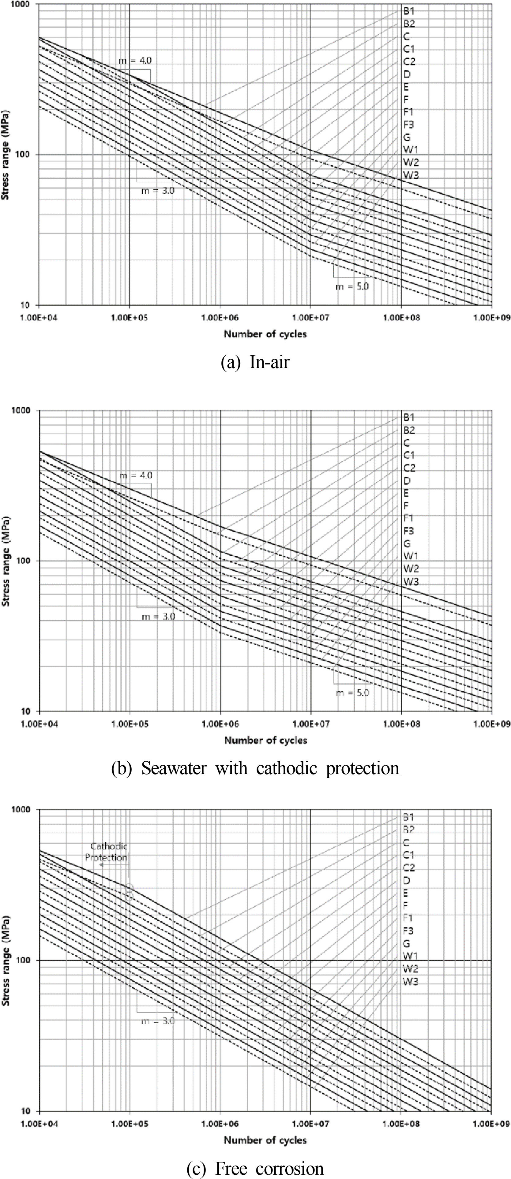
DNV GL defines the basic design S-N curves using the following Eq. (6), where slogN is 0.2 for weld joints of non-tubular and tubular members under an in-air environment (IA), a seawater environment with cathodic protection (CP), and a free corrosion environment (FC). In the case of high-strength steel with a yield strength exceeding 500 MPa, slogN is 0.162.
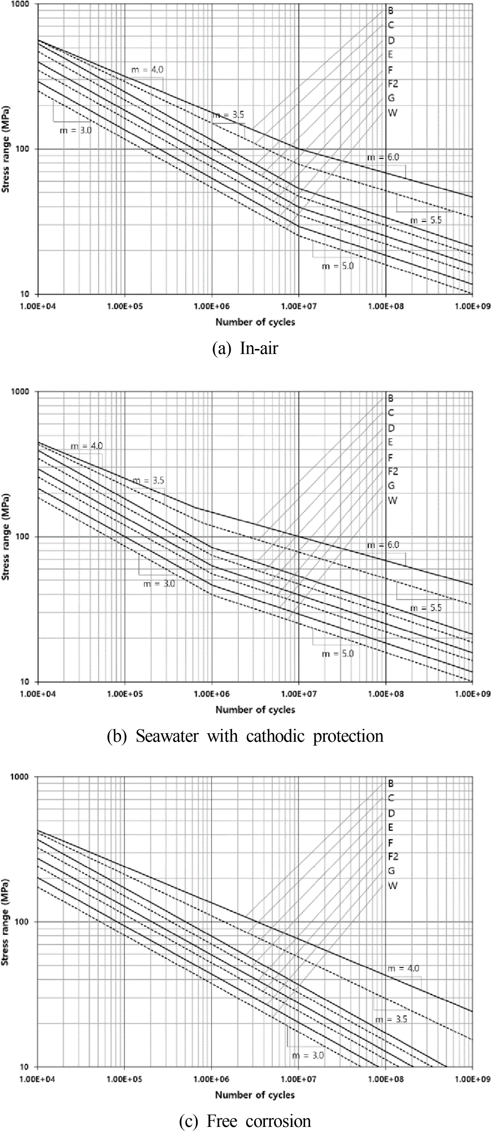
To select a basic design S-N curve that can be applied to a real offshore structure, the environmental conditions (IA, CP, and FC environments), SDC, type of stress (nominal, hot-spot, and effective notch stresses), and stress component (normal and shear stresses) should be determined. DNV GL provides the basic design S-N curves according to the environmental conditions and SDCs, whereas selection according to the type of stress is unclear. When using hot-spot stress, the D grade curve is recommended, regardless of the SDCs. Therefore, only the D grade curve has been used for hot-spot stress applications.
Tables 2,–4 summarize the material constants required in the basic design S-N curves corresponding to the environmental conditions of IA, CP, and FC, respectively. The basic design S-N curves for the IA and CP environments have two slopes. In addition, each curve contains the inherent SCF. As shown in Tables 2–3, the slope of the basic design S-N curve for the IA environment changes at 10 million cycles, but that for the CP environment varies at 1 million cycles. The intercept of the first slope for the CP environment is smaller than that for the IA environment.
The basic design S-N curve for the FC environment has a single slope. The single slope was assumed because the fatigue limit was ignored due to the stress corrosion effect. The basic design S-N curve for the FC environment does not include the inherent SCF. The SCF, which is strongly dependent on the structural shape, was not included due to the variability of the structural details under the FC environment.
Fig. 4 shows the basic design S-N curves corresponding to Tables 2,–4. Because the fatigue strength of the weld joint cannot exceed that of the base metal, the C and C1 curves corresponding to the weld joints where they intersect the B1 curve are shown. In a similar principle, the C curve where it intersects the B1 curve is shown because the C curve joins the B1 curve at 10,399 cycles.
The second intercepts of the basic design S-N curves corresponding to the IA and CP environments are identical, so the basic design S-N curves over 10 million cycles coincide with each other, as shown in Fig. 4(a) and (b). On the other hand, there is an apparent difference in the fatigue strengths at less than 10 million cycles between the IA and CP environments. The fatigue strength in the FC environment is considerably lower than that in the CP environment. On the other hand, the fatigue strengths of the B1 and B2 curves for less than 98,401 cycles in the FC environment are greater than those in the CP environment.
4.2 Basic Design S-N Curves of ABS
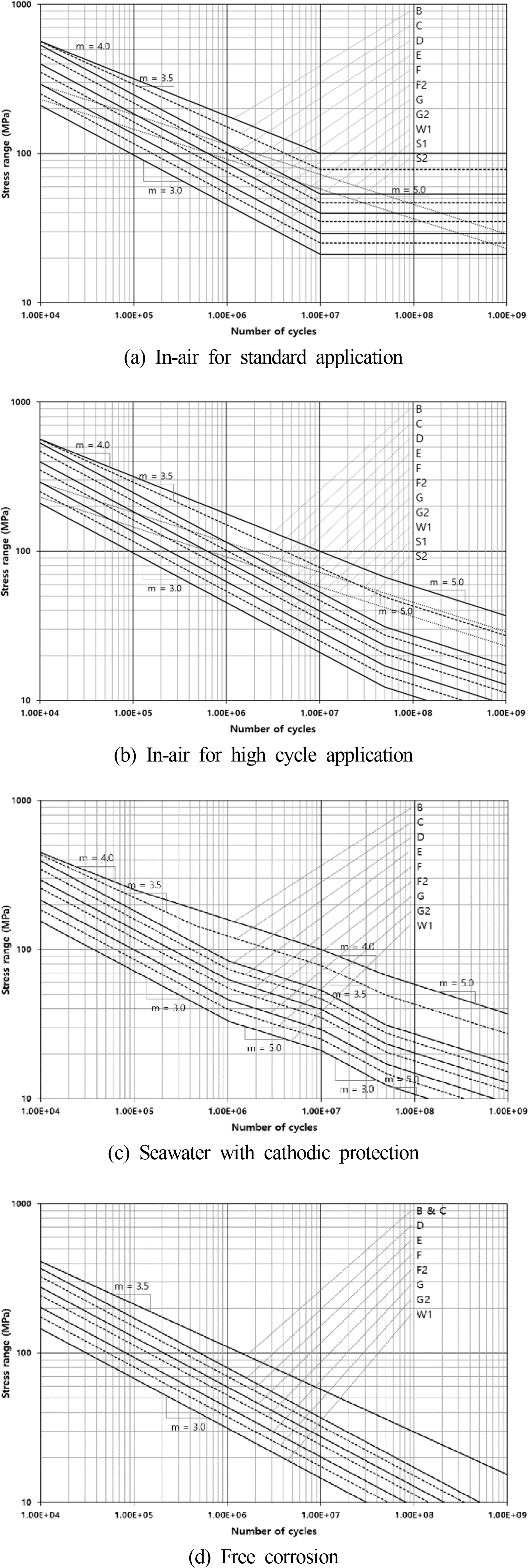
The basic design S-N curves of ABS are similar to those of DNV GL, but the SDCs of ABS are simpler. The SDCs for non-tubular joints defined by ABS are B, C, D, E, F, F2, G, and W, while DNV GL RP-C203 has 14 SDCs. Let NQ be the number of cycles to fatigue failure. The basic design S-N curves corresponding to the cases where the number of failure cycles are smaller and larger than NQ are expressed as Eqs. (7) and (8), respectively.
ABS provides the basic design S-N curves according to the environmental conditions and SDCs, but the advice for selecting the type of stress is unclear, which is similar to DNV GL. ABS recommends the E curve be used as the basic design S-N curve for hot-spot stress applications.
Tables 5,–7 and Fig. 5(a)–(c) present the material constants required for the basic design S-N curves corresponding to the IA, CP, and FC environments, respectively. The basic design S-N curves in the IA and CP environments are doubly sloped. As shown in Tables 5–6 and Fig. 5(a)–(b), the curve slopes in the IA environment change at 10 million cycles, but two curves in the CP environment intersect at approximately 1 million cycles (to be exact 1,010,000 cycles), excluding the B and C curves.
Comparing ABS and DNV GL, the standard deviation of log N in DNV GL, which is denoted as slog N, is constant regardless of the SDCs, but those in ABS, log σ, vary with the SDCs, which were copied from Almar-Næss (1985) and BS.
4.3 Basic Design S-N Curves of BS
The basic design S-N curve of BS is expressed as the slope (m) and intercept (logCd), as shown in Eq. (9). Table 8 lists the d value according to the probability of failure. For example, if the probability of failure is 2.3%; d equals 2.0 and Cd corresponding to this d becomes C2.
For the relative comparison between the codes, d was assumed to equal 2.0 for the BS S-N curves. Tables 9, -11 list the material constants for the three environments (the IA, CP, and FC). In Table 9, SOC is the fatigue limit at 10 million cycles except for the S1 and S2 grades. Therefore, the IA environment S-N curves show an infinite life after 10 million cycles. BS also presents the S1 and S2 grades under shear stress conditions. S1 is used if fatigue cracking occurs in the weld toes, while the S2 is used for weld throats.
Table 10 lists the material constants of the S-N curves under the CP environment, which was more complicated than those by the other codes. The three fatigue strength points (Srt, SOC, and SOV ) are the slope change points, where the Srt is listed in Table 10. The SOC and SOV are the fatigue strengths corresponding to 10 million and 50 million cycles, respectively. The S-N curves in the CP and FC environments cannot be applied to the cases under shear stresses.
Table 11 presents the basic design S-N curves in the FC environment, where they have single slopes like those in DNV GL and ABS.
Fig. 6(a) shows the basic design S-N curves in the IA environment. The fatigue life at low stress or high cycles in ships or offshore structures under variable loadings can be calculated after the fatigue strength SOV corresponding to 50 million cycles. A bilinear S-N curve can be applied to variable loading conditions because the variable stress may sometimes exceed the fatigue limit, even though the average stress is less than the fatigue limit. For example, assuming that the second slope is 5 (m=5), the S-N curve can be obtained, as shown in Fig. 6(b).
Because the slopes of the S-N curves in the CP environment change at three fatigue strength points, each S-N curve must show a total of four lines (see Fig. 6(c)). Fig. 6(d) shows that the S-N curve in the FC environment has a single slope.
Unlike DNV GL, ABS, BS can select the basic design S-N curves by comprehensively considering the structural shape, stress component (normal and shear stresses), stress type (nominal and hot-spot stresses), and potential crack direction. In particular, the S-N curves are so well structured that an engineer can easily pick an S-N curve for structural details either subjected to nominal stress or hot-spot stress. Hence, BS is recognized as a code that can minimize human errors.
4.4 Basic Design S-N Curves of IIW
Unlike DNV GL, ABS and BS, IIW uses the fatigue strength (FAT) at 2 million cycles and the corresponding slope to define the basic design S-N curves. The basic form of an S-N curve is expressed in Eq. (10). Eq. (12) was obtained by calculating C using equation (11) and substituting it into Eq. (10).
IIW provides the basic design S-N curves for aluminum and steel, but this paper concentrates on only the S-N curves for steel. The value of FAT determines the SDC of the basic design S-N curve provided by IIW. All basic design S-N curves can be applied to the IA condition. In the case of the CP or FC environment, it was stated that the strength level of the basic design S-N curve could be reduced by up to 70%. On the other hand, it is difficult to apply the basic design S-N curve of IIW in the case of non-IA environments.
IIW provides the basic design S-N curves using nominal stress, hot-spot stress, and effective notch stress. The S-N curve by stress components was also provided. That is, thirteen and two basic design S-N curves are provided for the normal and shear stress conditions, respectively. FAT80 and FAT100 are for problems under a shear stress, while normal stress should be applied to FAT36 to FAT160.
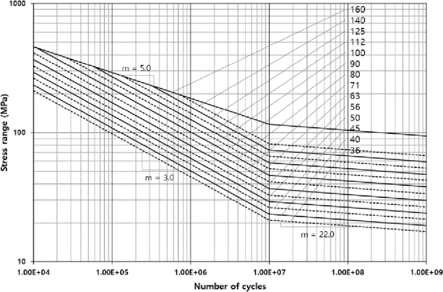
As shown in Table 12, the basic design S-N curves over 10 million cycles for the normal stress application have either a fatigue limit, or a slope of 22.0. Fig. 7 includes the basic design S-N curves based on normal stress with the second slope m=22.0. The basic design S-N curves for the shear stress application can be considered to be single sloped because they have a fatigue limit of 100 million cycles.
IIW provides the following two approaches to construct the basic design S-N curve for the hot-spot stress application. For the first approach, among the nine structural details presented in Table 13, it is important to select a structural detail that is most similar to the welded part of the target structure. An S-N curve corresponding to the selected structural detail should then be chosen. For most of the structural details, the applicable grades are only FAT100 or FAT90, as listed in Table 13.
The second method is to construct a new basic design S-N curve after revising FAT through finite element analysis. The following gives a summary of the process.
- Out of the 83 SDCs in the IIW code, select a reference structure detail, which should be most similar to the target.
- Derive two hot-spot stresses through finite element analyses for two structural details: σhs,ref and σhs,assess corresponding to the reference structural detail and target one.
- Derive a new FAT (FATassess) based on the ratio of the hot-spot stresses using Eq. (13).
-To construct a new basic design S-N curve using the FATassess.
The SDC should be FAT225 for effective notch stress applications. A basic design S-N curve can be constructed using a single slope (m =3.0).
4.5 Basic Design S-N Curves of EC3
EC3 provides the basic design S-N curves for steel. All curves can be applied to an IA environment and cannot be used in the CP or FC environment.
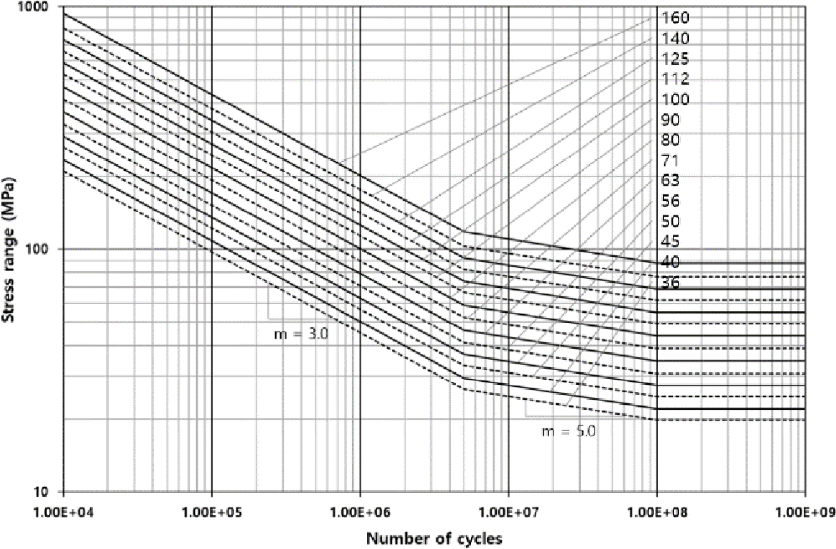
In the same way as the SCD by IIW, EC3 refers to the fatigue strength corresponding to 2 million cycles as ΔσC . EC3 determines the SDC based on ΔσC . For intervals less than 5 million cycles, the slope is 3.0. The fatigue strength at 5 million cycles is defined as ΔσD . The slope from 5 million cycles to 100 million cycles is 5.0. The fatigue strength at 100 million cycles is defined as ΔσL, which is the fatigue limit.
5. Comparison between Codes
5.1 Comparison of Nominal SDCs
The nominal grades in the IA environment are divided into two groups because some codes do not provide S-N curves in the CP or FC environment, as listed in Table 14. Here, the BS family includes DNV GL, ABS, and BS, while the IIW family refers to IIW and EC3.
Although the 14 SDCs are classified in the same group, some SDCs are used only in specific codes. Hence, Table 14 cannot be a perfect comparison table.
5.2 Comparison of the Probabilities of Failure
As previously explained, DNV GL and ABS use two standard deviations, so the probability of failure of the basic design S-N curves is 2.3%. If d = 2.0, the S-N curves of BS also have the same probability of failure as DNV GL and ABS. On the other hand, IIW and EC3 provide the S-N curves with a 5% probability of failure (refer to Table 15).
5.3 Comparison of the S-N Curves
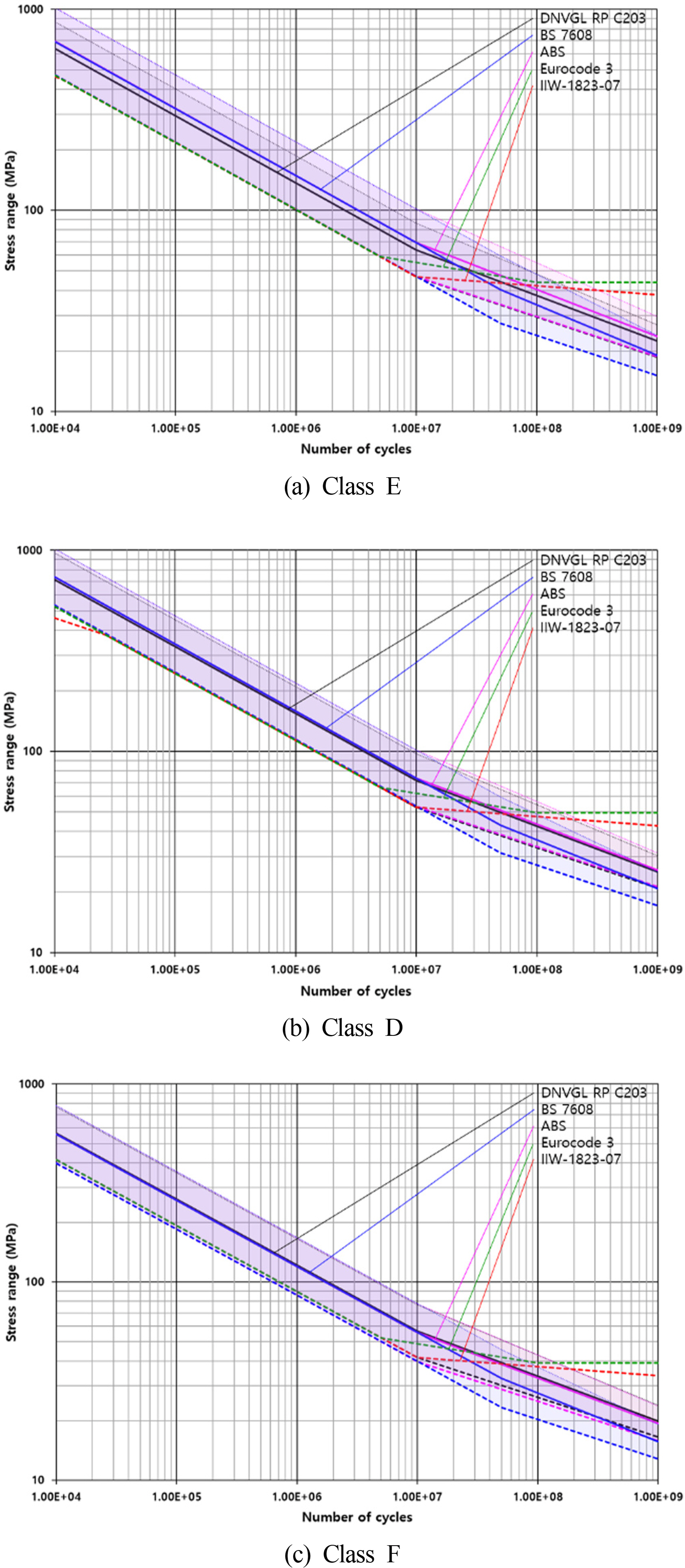
The S-N curves in the IA environment were compared because the S-N curves of some codes cannot be used in the CP or FC environment. The S-N curves of the D-, E-, and F grades were compared. Fig. 9 presents the S-N curves corresponding to the mean, +2 standard deviations, and -2 standard deviations as thick solid lines, thin dotted lines, and thick dotted lines, respectively.
5.3.1 Grade E or FAT80
The E grade of the BS family and the FAT80 grade of the IIW family are equivalent to each other; Fig. 9(a) shows the S-N curves for the grades. The E grade mean curves by ABS and BS are the same up to 10 million cycles. Up to the same life, the mean curves by DNV GL were lower than those by ABS and BS. Therefore, the average S-N curves of DNV GL were the most conservative for 10 million cycles among the E grade curves belonging to the BS family. The mean S-N curve by BS was the most conservative for the long life of over 10 million cycles.
The basic design S-N curves (-2 standard deviation curves) of the BS family coincide until 5 million cycles. The BS curve is the most conservative after 10 million cycles, while the basic design S-N curves by DNV GL and ABS are the second most conservative. The EC3 curve is most optimistic after 10 million cycles.
5.3.2 Grade D or FAT90
The grade D of the BS family and the FAT90 of the IIW family are equivalent. Fig. 9(b) presents the S-N curves in the IA environment. The mean S-N curves by the five codes are similar up to 10 million cycles. If it exceeds 10 million cycles, the mean S-N curve by BS is the most conservative. As with the grade E, the three basic design S-N plots by the BS family were identical for up to 5 million cycles. Above 10 million cycles, the BS basic design curve was the most conservative.
5.3.3 Grade F or FAT71
The grade F of the BS family is equivalent to the FAT71 of the IIW family. Fig. 9(c) shows the IA environment S-N curves. The trend of the F grade curves by the codes was similar to that in the D grade curves.
6. Conclusions
This paper analyzed the characteristics of the S-N curves according to various industry standards and codes to provide guidelines for applying the appropriate codes when designing ships and offshore structures. The S-N curves of the five codes (DNV GL, ABS, BS, IIW, and EC3) were analyzed and compared for the non-tubular members made from steels.
Before the code-by-code comparison, the notations and symbols were summarized into a single table by each code to minimize confusion.
Unless stated otherwise, the S-N curves presented in most codes were based on the nominal stress. On the other hand, because the hot-spot stress has been used mainly in the design of offshore structures, it is important to select a basic design S-N curve for a hot-spot stress application problem code by code. In addition, a method of evaluating hot-spot stresses was introduced.
DNV GL, ABS, and BS define an S-N curve with an intercept and slope, while IIW and EC3 describe it with a fatigue strength at 2 million cycles and a slope. An examination of the probability of failure for each code, DNV GL, ABS and BS used a basic design S-N curve based on a failure probability of 2.3% and those corresponding to a 5% failure probability by IIW and EC3.
The material constants of the basic design S-N curves presented in each code were arranged in a table so that the reader can easily use them. The corresponding S-N curves are provided graphically so that a design engineer can apply them without needing to read the complex codes fully.
The nominal grades by the BS family (DNV GL, ABS, and BS) and IIW family (IIW and EC3) were tabulated to enable a relative comparison. In addition, the mean and basic S-N curves by the five codes were compared for the E, D, and F grades. Overall, the BS presented the most conservative basic design S-N curves.
Part 1 of this paper compared the basic design S-N curves. Part 2 discussed various factors influencing the basic design S-N curves. Nevertheless, because this paper targeted the non-tubular steel members, it will be necessary to deal with tubular members in future studies.