
1. Introduction
According to the National Oceanic and Atmospheric Administration (NOAA), the Earth’s average temperature is increasing annually as global warming continues, and the temperature of the Arctic region is increasing twice as fast as those of other regions (NOAA, 2018). With Arctic glaciers melting owing to global warming, the importance of developing marine resources buried in the Arctic is emerging. According to the United States Geological Survey, undiscovered recoverable resources in the Arctic region include approximately 90 billion barrels (Bbbl) of oil, 1,669 trillion cubic feet (Tcf) of gas, and 44 Bbbl of natural gas liquid (Bird et al., 2008). It is estimated that 13% of the world’s undiscovered oil volume and 30% of the world’s undiscovered gas volume are buried in the Arctic region. In general, marine resources in the deep sea are developed by offshore structures, and it is important to collect and analyze the metocean data of sea areas where marine resources are buried for the operation and survival of offshore structures. Metocean data include wave, wind, current, water depth, tide, and soil conditions. To reflect metocean data in the design of offshore structures, extreme value analysis should be conducted (API, 2005). Metocean data can be collected from measurement data of actual sea areas that use buoys or ships, hindcast data that estimate the desired data of the past through numerical methods based on past metocean data, and satellite data that use satellites. According to DNVGL (2015), for the design of offshore structures, the significant wave height (Hs) and spectral peak wave period (Tp) of 100-year return values should be used for waves, whereas the 100-year return value of the one-hour average wind speed at 10 m above the mean sea level (MSL) should be used for wind speed. For ocean currents, the 10-year return value of the current speed should be reflected in the design.
To derive return values through statistical methods, methods for selecting the collected data must be determined. Such methods can be primarily categorized into global and event models. Global models include the initial distribution and total sample methods that use the entire data statistically, and the event models include the peak over threshold method, which uses data above a certain threshold, and the annual maxim method, which uses only the annual maximum values (DNV, 2014).
Extreme value distributions (EVDs) used for extreme value analyses include the Gumbel, Frechet, Weibull, and log-normal distributions. Methods for estimating the parameters of EVDs include the method of moment, maximum likelihood estimation, and least-squares method (DNV, 2014). Jeong et al. (2004) conducted extreme value analyses using Weibull, Gumbel, Log-Pearson type-III, and log-normal distributions using the Hs data of approximately 20 years obtained from 67 ocean stations in South Korea. They provided design wave height information in the deep-sea for the return period of 50 years and suggested that Gumbel distribution was the most suitable method. In addition, they provided the extreme highest tide level information for each return period by conducting an extreme value analysis through generalized extreme value, Gumbel, and Weibull distributions using the extreme highest tide level data of 23 tide stations on the coast of South Korea, and they suggested that Gumbel distribution was the most suitable method (Jeong et al., 2008). Ko et al. (2014) developed a numerical wind speed model that numerically implemented typhoons for four locations on the west coast of the Korean Peninsula (Gunsan, Mokpo, Jeju, and Haemosu No. 1) and presented extreme wind speeds for the four locations by applying the Gumbel distribution and estimating parameters through the probability weighted moment method.
EVDs were applied to various metocean data. In the case of wave data, however, Hs and Tp were important design elements for the design of offshore structures. DNVGL (2017) and BV (2015) recommended the use of the inversed first order reliability method (I-FORM), which used the joint distribution of EVDs, to obtain the return values for Hs and Tp.
In this study, the metocean data (wave, wind, and current) of the Barents Sea in the Arctic region were collected. In addition, for the extreme value analysis of the wave data, return values were calculated using I-FORM, which used the joint distribution of the marginal probability distribution for Hs (Gumbel distribution and two- and three-parameter Weibull distributions) and the conditional probability distribution of Tp for the given Hs (log-normal distribution) (DNVGL, 2017; BV, 2015; Choi, 2016). For the wind and current speeds, which are single variables, extreme value analysis was conducted through the Gumbel distribution and two- and three-parameter Weibull distributions. The least-squares method was used for parameter estimation, and the Kolmogorov-Smirnov (K-S) test was applied as the goodness-of-fit test. Through these processes, the return values for Hs, Tp, wind speed, and current speed required for the design of offshore structures to be operated in the Barents Sea were derived.
2. Metocean Data Collection and Analysis
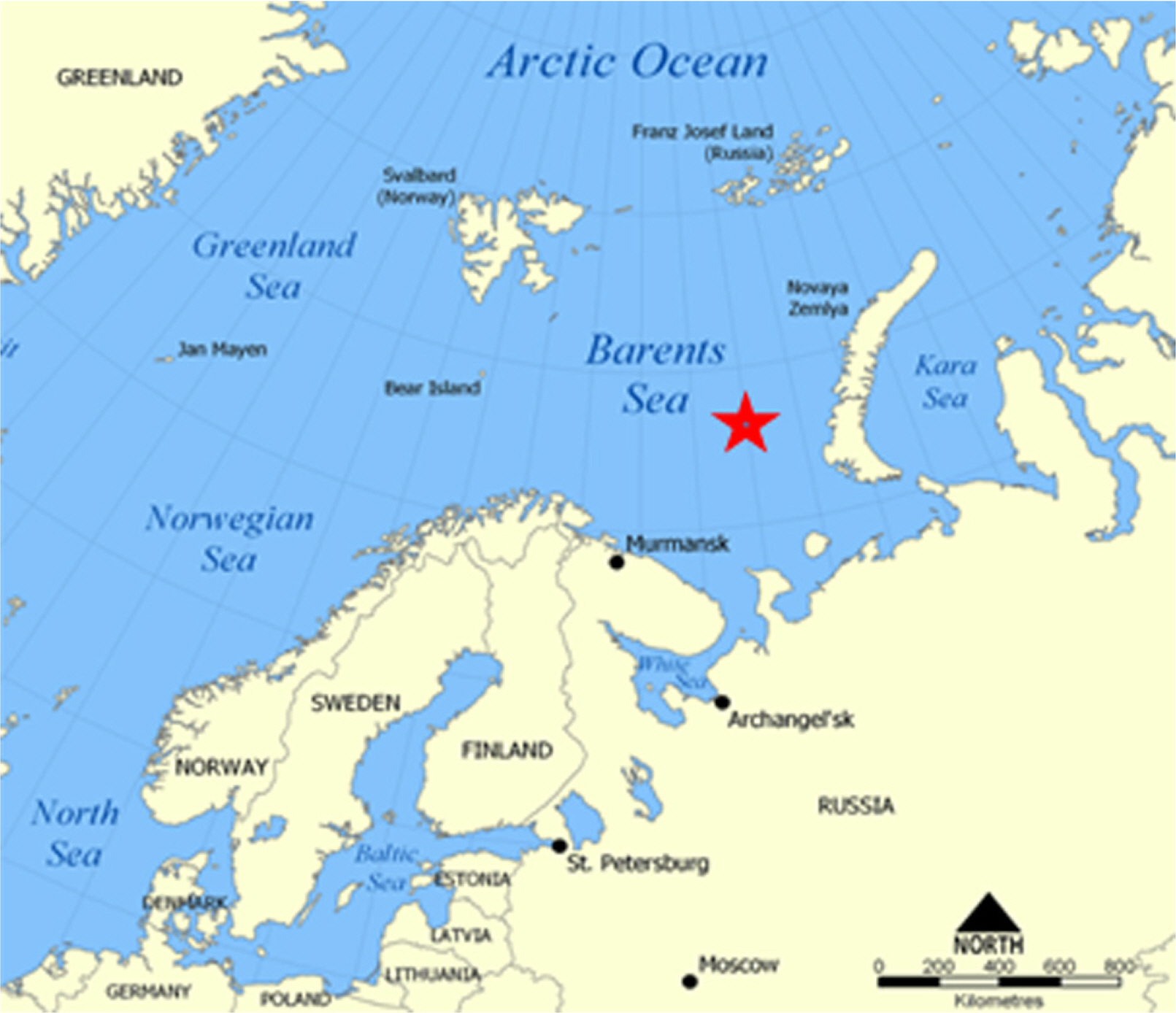
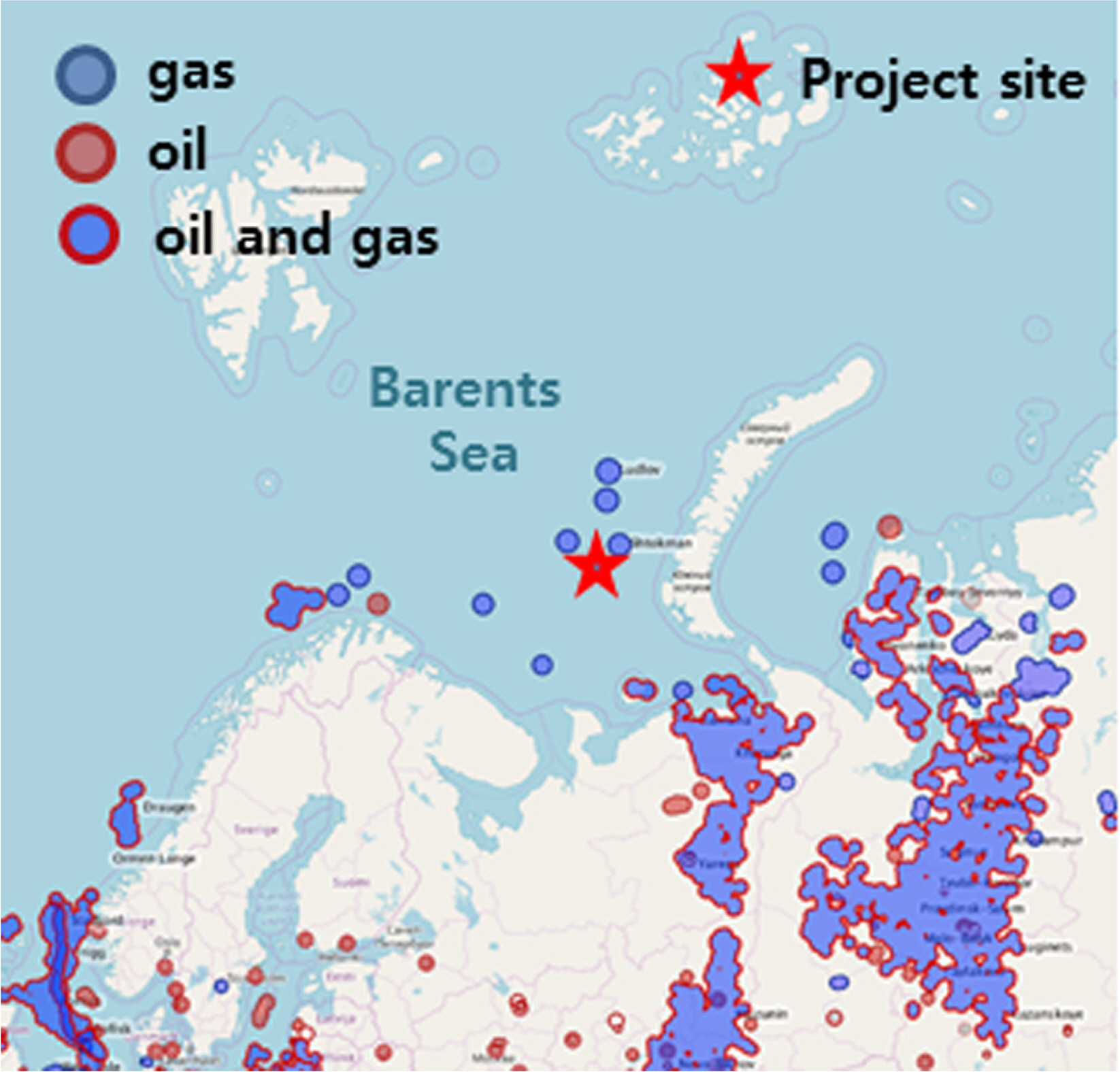
The project site (Fig. 1) is the Barents Sea of water depth 258 m (latitude: 73N and longitude: 44E), where gas fields were distributed around the site (Fig. 2). For the wave (Hs, Tp, and wave direction), wind (wind speed and wind direction), current (current speed and current direction), and an ice floe thickness data, the hindcast datasets of Global Reanalysis of Ocean Waves 2012 (GROW2012) from Oceanweather Inc. were purchased. In the hindcast datasets of GROW2012, wave and wind models provided by the General Bathymetric Chart of the Oceans and Climate Forecast System Reanalysis were used to estimate the data for waves, wind, current, and ice floe (Oceanweather Inc.).
To conduct the extreme value analysis, the consistency, period, and validity of the collected data must be examined first (Van Os et al., 2011). Compared with the measurement data, the hindcast data have no possibility of missing data and generating outliers owing to typhoons or defects in the measuring equipment and can secure a data period irrespective of the installation time of the measuring equipment. The wave and wind data were recorded at one hour intervals for a decade from January 2007 to December 2016, and the current data were recorded in the water depth direction at one day intervals for two decades from January 1993 to December 2012. The ice floe thickness data during the same period as that of the current data were provided, but it was discovered that no ice existed in the project site.
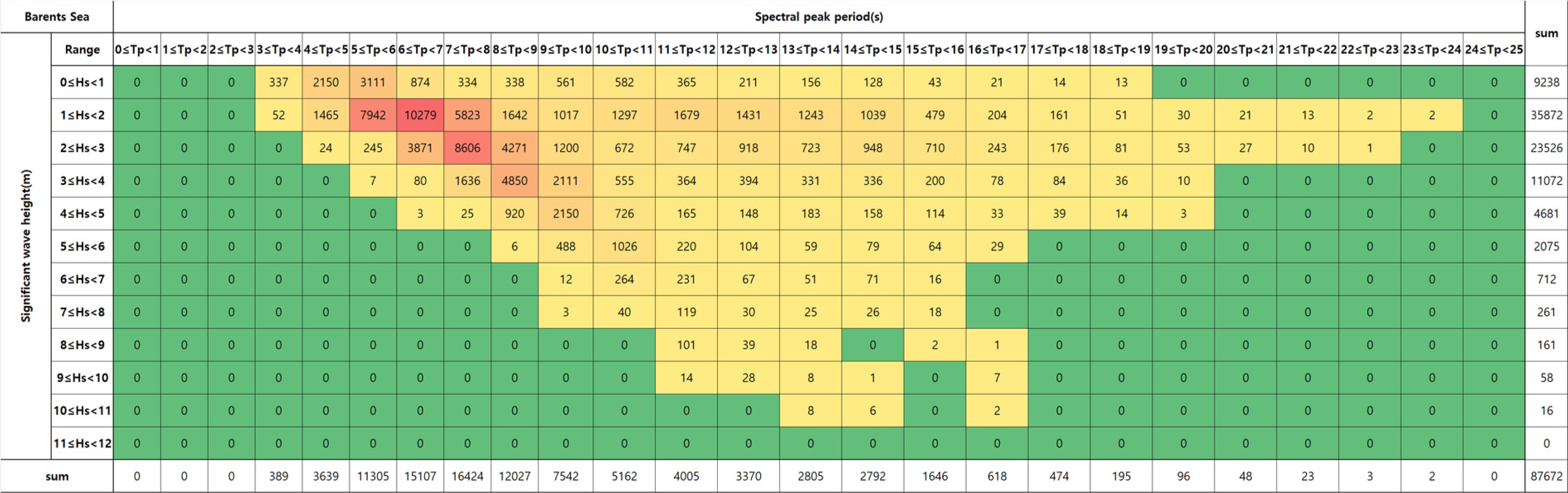
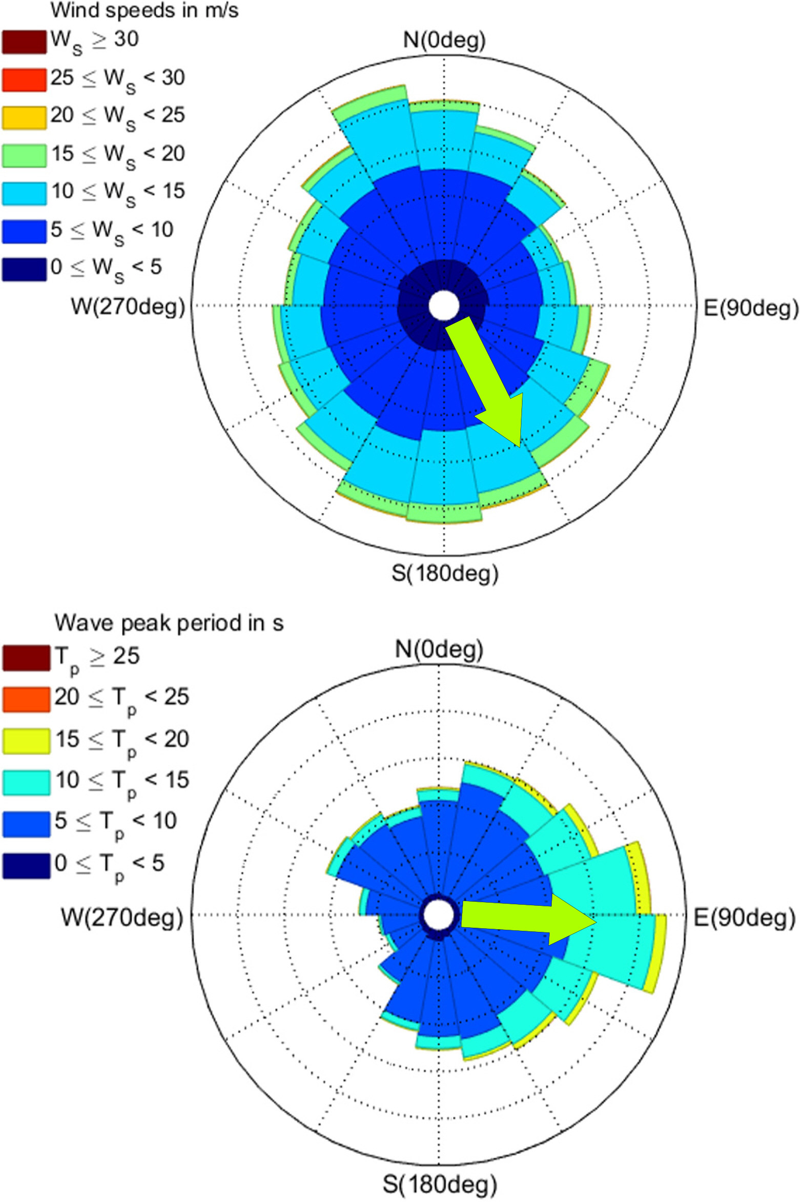
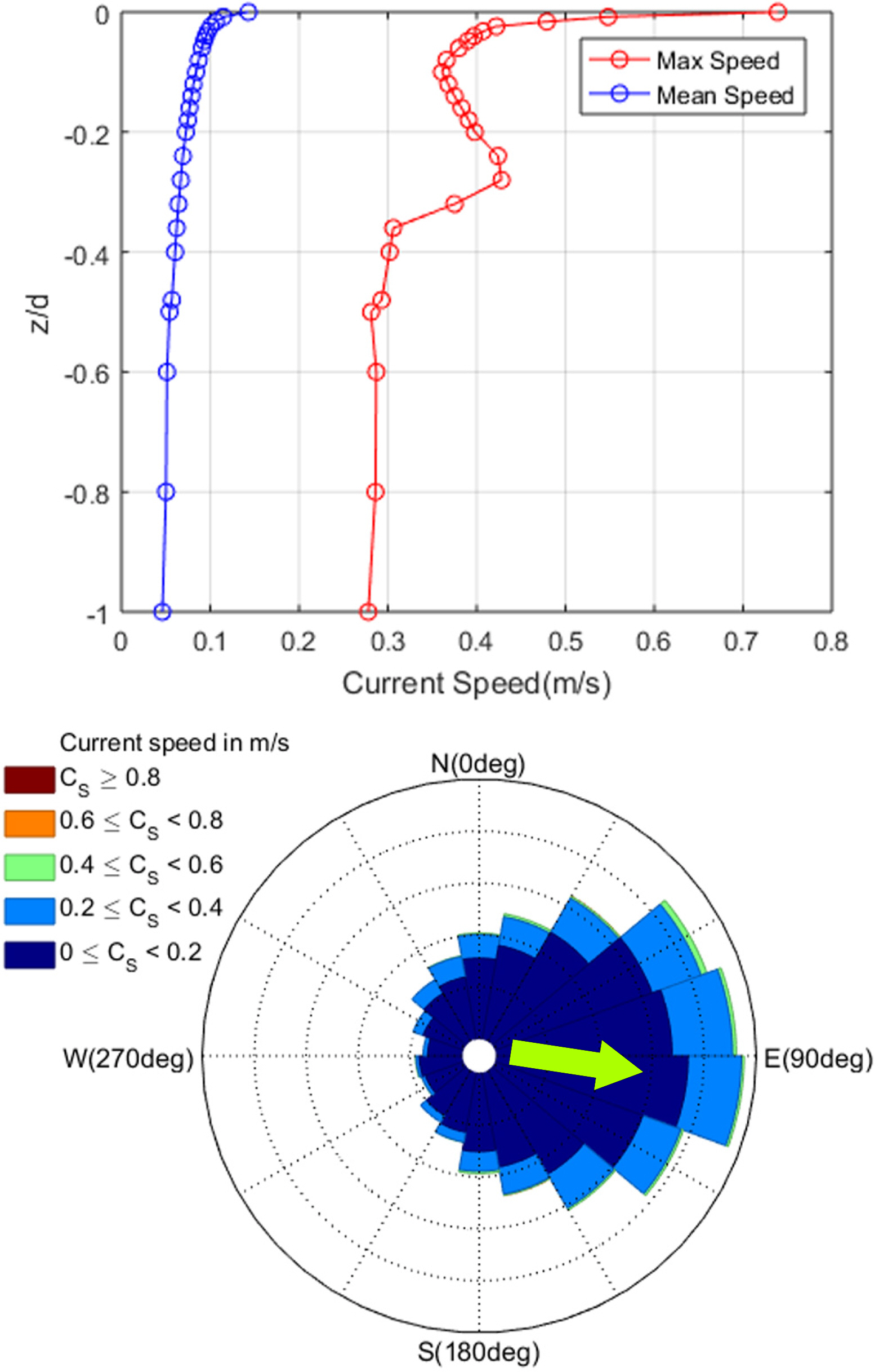
The wave data showed the wave scatter diagram (WSD) for Hs and Tp; the wave rose for the wave direction and Tp, and the wind data showed that the wind rose for the wind direction and wind speed (Ws) (Figs. 3 and 4). The current data represented the current increase for the current direction and current speed (Cs) at the surface and the current profile in the water depth direction (Fig. 5).
The WSD showed frequencies at 1 m intervals for Hs and at 1s intervals for Tp, and the total number of data was approximately 87,600. The wave conditions with the highest frequencies in the project site were 1–2 m for Hs and 6–7 s for Tp. The wave, wind, and current directions could be confirmed through the rose diagrams, and the directions were categorized into east (90°), south (180°), and west (270°) in the clockwise direction from the north direction (0°). In the case of the hindcast data purchased from Oceanweather Inc., the wave and current directions were defined as the directions to which the wave and current were moving, while the wind direction was defined as the direction from which the wind was coming. The wave and wind directions with the highest frequencies were East and North Northwest (Fig. 4). Fig. 5 shows the current speed profile and direction in the water depth direction (z). The current speed profile was nondimensionalized with the water depth of the project site (d). The average and maximum current speeds were the fastest at the surface, and the dominant current direction at the surface was from the West to the East.
3. Extreme Value Analysis
For the extreme value analysis of metocean data, data collection, data selection, EVD selection, parameter estimation method selection, goodness-of-fit test, and return value derivation are required (Mathiesen et al., 1994). In this study, a global model that utilizes all of the collected metocean data was selected. In addition, the Gumbel distribution, two- and three-parameter Weibull distributions, and log-normal distribution were used as EVDs. The least-squares method was used to estimate the parameters of the EVDs. As the goodness-of-fit test, the K-S test that uses the maximum distance as a test statistic by comparing the cumulative distribution function (CDF) of metocean data with that of each EVD was used (Jeong et al., 2004; Jeong et al., 2008).
Hs is the significant wave height; α, β, and γ are the scale parameter, shape parameter, and location parameter, respectively.
Tp is the spectral peak wave period, and Φ is the CDF of the standard normal distribution (eq. (5)).
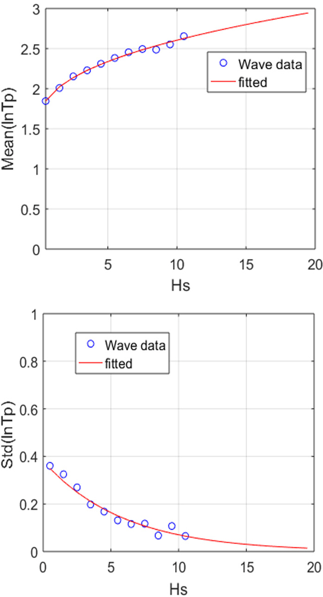
μ of the log-normal distribution can be expressed with the average value of ln(Tp), as shown in Eq. (6); σ can be expressed with the standard deviation of ln(Tp), as shown in Eq. (7) (DNV, 2014).
To estimate the parameters and coefficients (a0, a1, a2, b0, b1 and b2) using the least-squares method, taking the log of both sides of each EVD, the log-normal distribution average equation, and the standard deviation equation followed by summarizing them into linear equations result in Eqs. (8)–(12).
For Eqs. (8) and (9), the least-squares method can be used directly. For Eq. (10), however, the parameters for which the R2 value was closest to 1 were estimated, while the value of γ was changed approximately 1,000 times within the range in which the value in the log was not negative. The R2 value is the coefficient of determination that indicates the goodness-of-fit corresponding to the regression line. It approaches 1 as the samples used in statistical analysis exhibits smaller errors with the regression line.
Once the parameters are obtained through the least-squares method, the return values can be obtained using Eqs. (13)–(16).
After changing the variable from Hs to wind speed and current speed, their return values were derived using the same method as presented above.
3.1 Extreme value analysis on wave and results
Hs and Tp, which are wave data, can be expressed by the conditional modeling approach, and the joint probability distribution of the two variables can be expressed as the product of the marginal probability distribution of Hs and the conditional probability distribution of Tp for a given Hs (Orimolade et al., 2016; DNVGL, 2017).
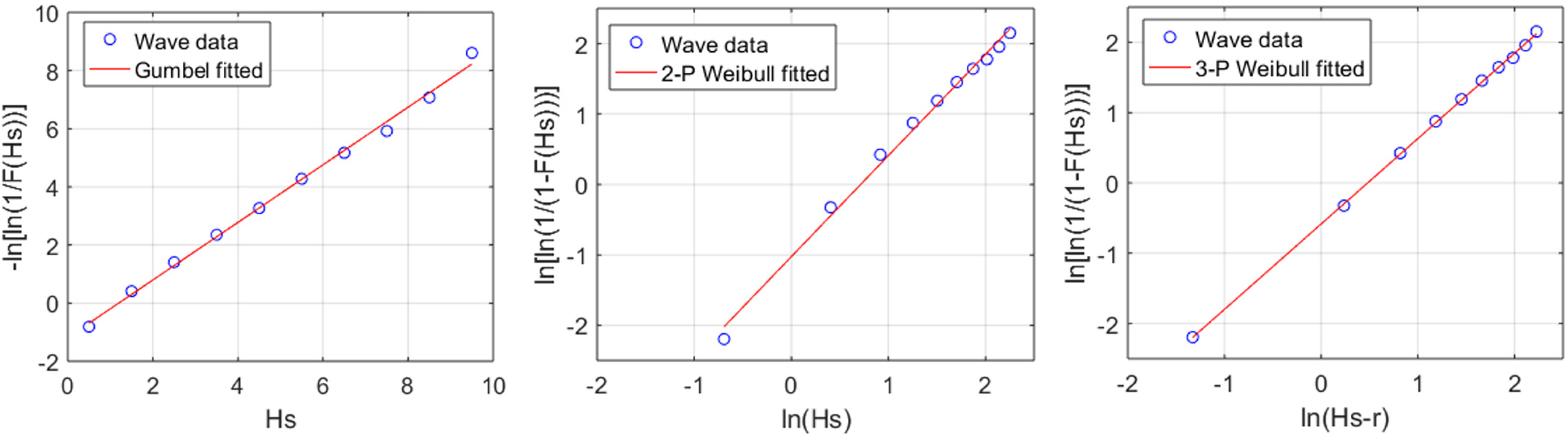
In this study, the marginal probability distribution of Hs was assumed to be a Gumbel distribution and two- and three-parameter Weibull distributions using the WSD and the conditional probability distribution of Tp, as the given Hs was assumed to be a log-normal distribution to calculate return values using the I-FORM method. Extreme value analysis was conducted after transforming the EVDs from the probability distribution function form to the CDF form for the convenience of calculation. The I-FORM method was proposed by Winterstein et al. (1993), and the data of Haver and Nyhus (1986) were used for the parameter estimation equations of the EVDs used. In other words, the I-FORM method calculates the exceedance probability in advance and obtains the corresponding response rapidly.
Q is the exceedance probability. It is the reciprocal number of N, which is the total number of data.
where F (Hs) is the CDF of the marginal probability distribution, and F (Tp|Hs) is the CDF of the conditional probability distribution
EVDs are moved to the space of the standard normal distributions of u1 and u2.
A circle equation with a radius of B was introduced and represented by the relationship between the short-term period (Tss) an return period (Tr).
where B is the reliability index. One hour was used for Tss, Tr is the return period; 1, 10, and 100 years were used.
si in Eq. (21) is a dummy index, i.e., a number in the section between −1.0 and 1.0. Once B is determined Hs and Tp can be obtained using the inverse function of each EVD (Eqs. (22)–(24)).
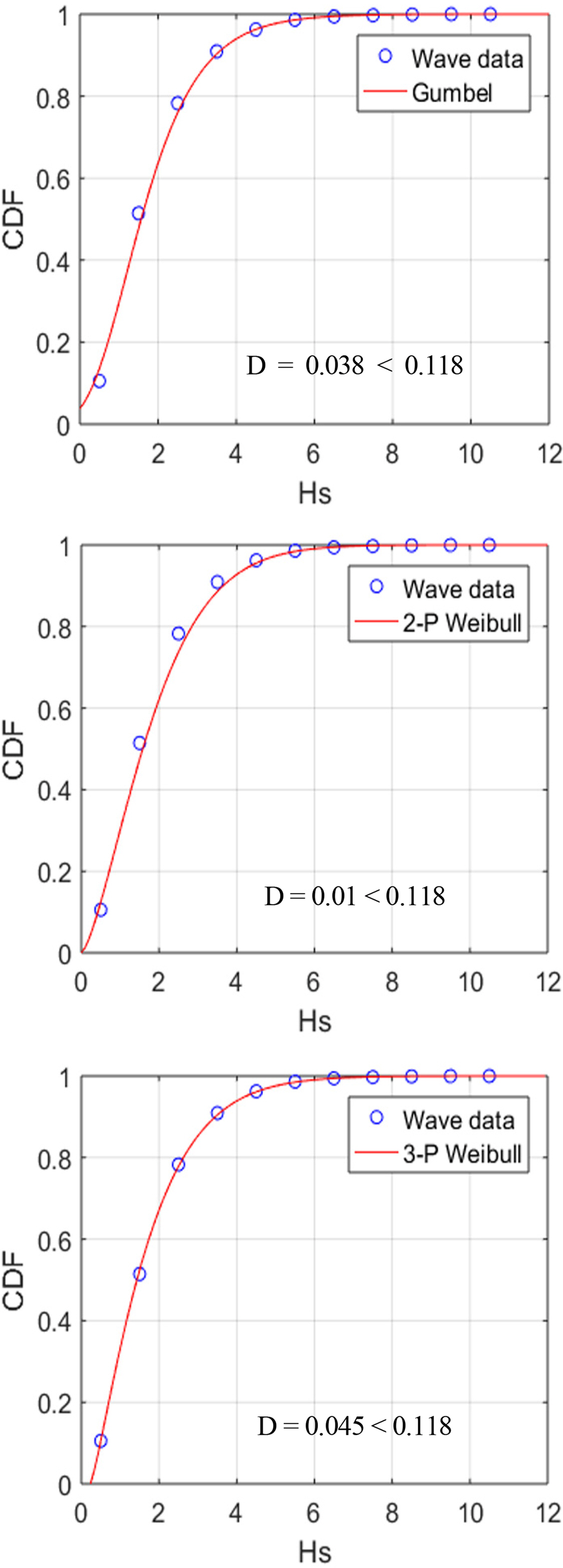
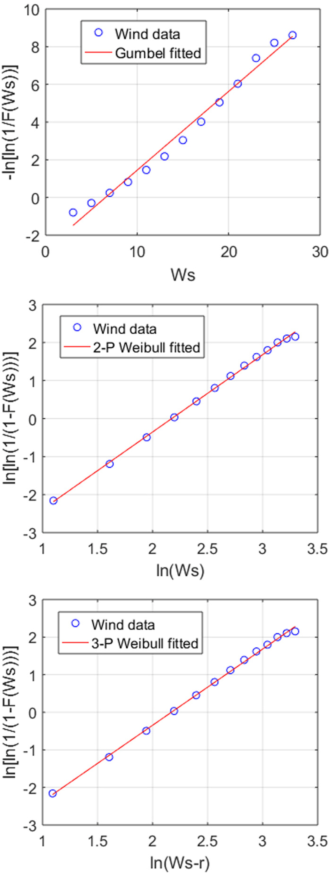
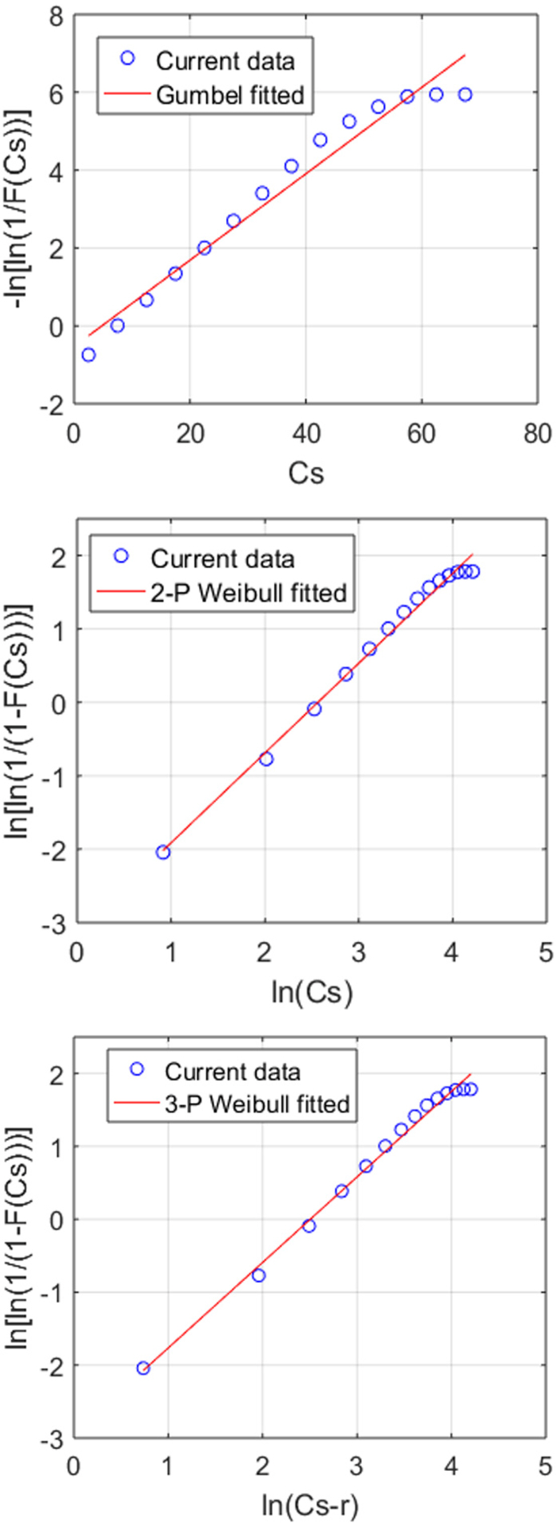
The parameters of each EVD were estimated using the least- squares method, and the goodness-of-fit was tested using the K-S test. The parameters for which the R2 value was the highest were extracted using MATLAB software (Figs. 6–7). The R2 value was 0.99, indicating that the numerical values agreed well with the actual values. The parameters were obtained using the slopes and y-intercept values (Tables 1–2).
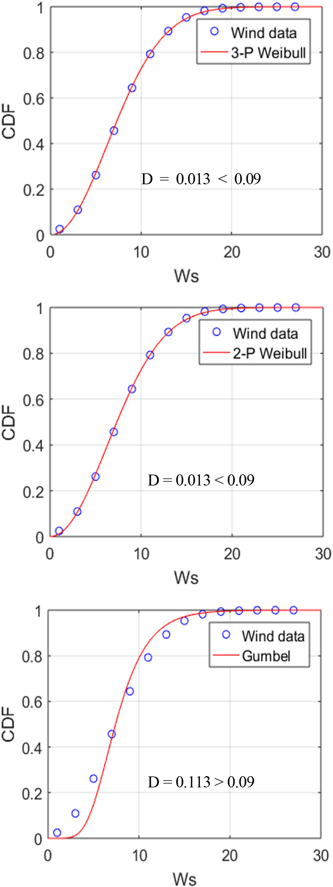
To test the estimated parameters, the maximum distance difference between the CDF of the wave data and the CDF that included the parameters obtained by the least-squares method is shown in Fig. 8. Based on the result of the K-S test, a test statistic (D) value is presented. If this value is smaller than the threshold (Dcri) of 0.118 by the number of wave data at the significance level of 5%, then the null hypothesis that no difference exists between the two CDFs mentioned above can not be rejected (Kanji, 2006). In other words, it was discovered that the graphs of CDFs, including the parameters, agreed well with the actual data.
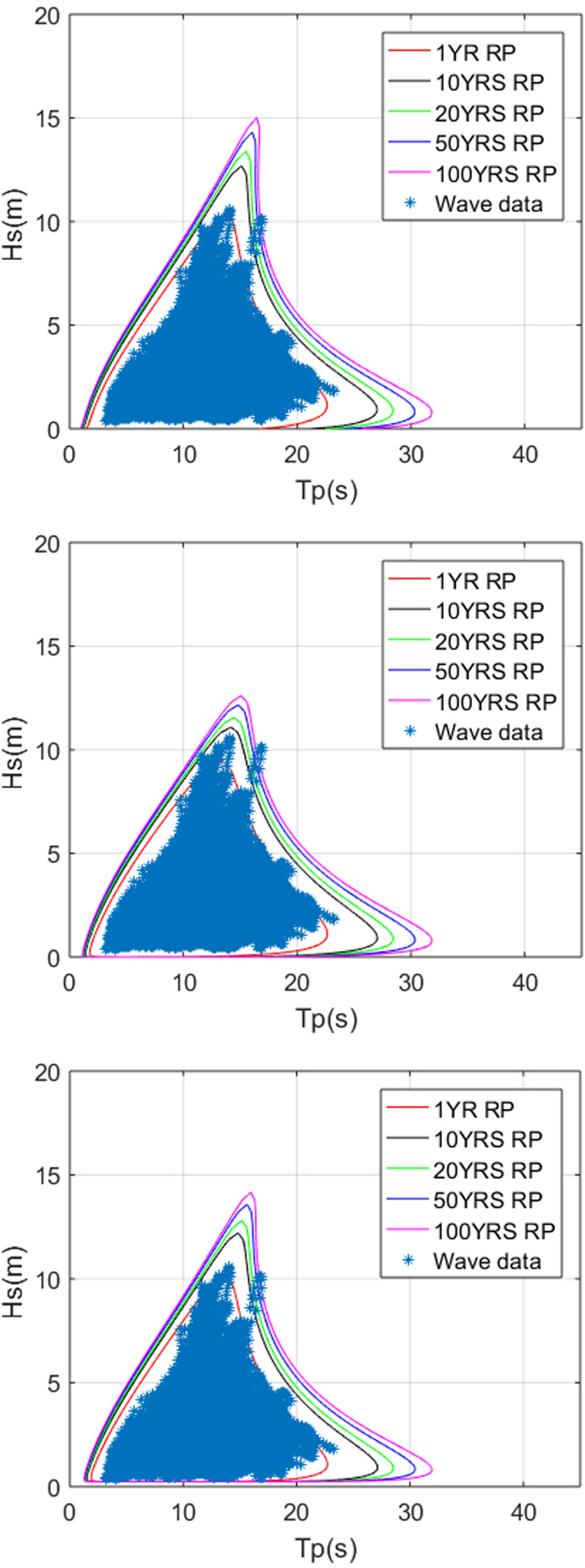
The contours for Hs and Tp were expressed using the I-FORM method of Eqs. (17)–(24), as shown in Fig. 9. The contours are shown for each return period (RP), and the return values corresponding to each return period are shown in Table 3.
When the 10-year hindcast data were compared with the 10-year return values, the highest prediction values could be obtained when the Gumbel distribution was assumed as the marginal probability distribution. The next highest values were derived by the three-parameter Weibull distribution, and two-parameter Weibull distribution exhibited the most similar results to those of the collected data. This was because the Gumbel distribution had a higher degree of scatter than the Weibull distribution. In addition, when the equations for obtaining the return values of the two- and three-parameter Weibull distributions were compared, it was discovered that different results were obtained depending on the value of the location parameter.
3.2 Extreme value analysis on wind and current and results
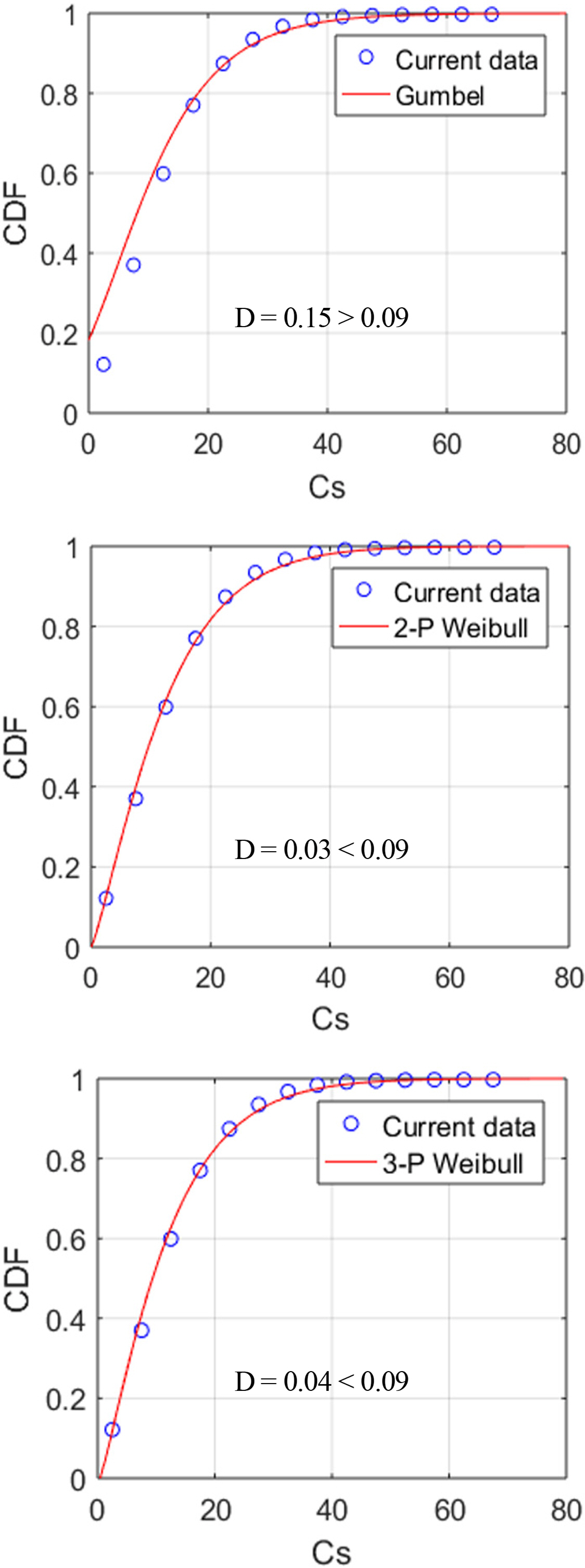
The wind speed (Ws) was distributed within the 0–27 m/s range and the total number of data was approximately 87,600. The CDF was obtained at 2 m/s intervals. The current speed (Cs) ranged from 0 to 70 cm/s and the total number of data was 7,200. The CDF was obtained at 5 cm/s intervals. To derive the return values for the Ws and Cs, which were single variables, the Gumbel distribution and two- and three-parameter Weibull distributions were used as EVDs, and the least-squares method was used for parameter estimation (Figs. 10 and 12). The parameters were obtained using the slopes and y-intercept values when the R2 value was the highest (Tables 4 and 6). The K-S test was used to test the parameters, and test statistic (D) values are presented as results (Figs. 11 and 13). If these values are smaller than the threshold (Dcri) of 0.09 by the number of wind and current data at the significance level of 5%, then the null hypothesis cannot be rejected. In other words, it was discovered that the graphs of the CDFs, including the parameters, agreed well with the actual data. The return values for the Ws and Cs were calculated using a method similar to the analysis of the wave data (Tables 5 and 7).
As for the overall tendency of the return values for the Ws and Cs, the Gumbel distribution exhibited the highest prediction values, similarly to the results of the wave data, followed by the three- and two-parameter Weibull distributions. When the maximum Ws and Cs of the 10-year hindcast data (27 m/s and 70 cm/s, respectively) were compared with the 10-year return values of the two-parameter Weibull distribution (29.07 m/s and 72.49 cm/s, respectively) large differences of 7.6% and 3.5% were discovered, respectively.
The prediction values of the Gumbel distribution were the highest because the null hypothesis was rejected as the test statistic was higher than the threshold in the K-S test results; hence, overestimated results were obtained. This was because the intervals determined to calculate the ranges and frequencies of the Ws and Cs were larger compared to the wave data; hence, errors were accumulated when the parameters were calculated using the least-squares method. The reclassification of data through the independent and identically distributed (IID) verification of changes in the intervals for extracting the frequencies of the Ws and Cs is expected to further improve the accuracy (Choi et al., 2019).
4. Conclusion
In this study, an extreme value analysis for the Hs, Tp, wind speed, and current speed was conducted using the hindcast metocean data of the Barents Sea in the Arctic region to derive return values required for the design of offshore structures. In the extreme value analysis for the Hs and Tp, the marginal probability distribution of the Hs was assumed to be a Gumbel distribution and two- and three-parameter Weibull distributions, and the conditional probability distribution of the Tp for the given Hs was assumed to be a log-normal distribution to calculate return values using the I-FORM method. For the Ws and Cs, which were single variables, return values were calculated through the Gumbel distribution and two- and three-parameter Weibull distributions. The parameters were estimated using the least-squares method and tested through the K-S test.
The return values for the Hs, Tp, and wind speed for the 100-year return period and those for current speed for the 10-year return period, which are required for the design of general offshore structures were summarized (as shown in Table 8). As the degree of scatter of metocean data increased, the differences in return values between the Gumbel and Weibull distributions increased. The Weibull distribution should be used for widely distributed metocean data, such as wind speed and current speed data.
The results of this study can be used as the metocean data design values of offshore structures to be installed in the Barents Sea; furthermore, they can be utilized as basic data for offshore structure motion and mooring analyses, structural analyses, and air gap calculations. In the future, the method of estimating parameters will be extended from the least-squares method to the moment area and maximum likelihood methods. In addition, in the case of widely distributed metocean data, such as Ws and Cs data, they will be reclassified through an IID verification to select appropriate intervals.