Article information

Abstract

1. 서 론

해양 유체를 이해하기 위하여 인류는 끊임없이 노력해왔다. 그 중 대표적인 성과가 Boussinesq 방정식이며 이는 천수 영역 (Shallow water)에서 파랑을 계산하는 수학적 모델이다. 따라서 지진해일, 항만, 잠제 등을 다루는 해양, 토목 공학에서 중요한 방정식이므로 많은 관련 연구가 진행되고 있다(Jang, 2017; Jang, 2018a; Jang, 2018b).

고전 Boussinesq 방정식(Boussinesq, 1872)은 평평한 해저 지형에서만 적용된다. 반면에 Peregrine 방정식(Peregrine, 1967)은 완만한 기울어진 해저 지형에 적용된다. 약한 비선형성(Weakly nonlinearity)과 약한 분산성(Weakly dispersivity)을 고려하는 Peregrine 방정식은 천수 영역에서는 비교적 정확한 결과를 도출하지만, 심수 영역(Deep water)에서는 다소 부정확한 결과를 도출한다. Madsen과 Sørensen(1992)은 이러한 제한성을 극복하기 위하여 Madsen-Sørensen 확장형 Boussinesq 방정식(1992)을 고안하였다(Madsen and Sørensen, 1992).

수치해석기법으로 여러 수학적 모델을 해석하는 것처럼 Madsen-Sørensen 확장형 Boussinesq 방정식(1992)도 수치해석기법을 통하여 해석 할 수 있다. Grilli et al.(1994)은 잠제를 지나는 고립파에 관한 실험을 하였으며(Grilli et al., 1994), Ghadimi et al.(2016)은 Madsen-Sørensen 확장형 Boussinesq 방정식(1992)을 유한요소법(FEM, Finite element method)으로 수치해석을 하여 이를 확인하였다(Ghadimi et al., 2016). Kang et al.(2017)은 1차원 Madsen-Sørensen 확장형 Boussinesq 방정식(1992)을 기존 수치 방법과 차별되는 Crowhurst and Zhenquan(2013)의 유한차분/수치계산법을 사용하여 평평한 해저 지형과 해안선을 포함하는 완만한 경사의 해안 지형(Peregrine, 1967)에서 고립파 전파(Propagation)와 오름(Shoaling)에 관한 수치 실험을 하였다(Kang et al., 2017).

본 연구에서는 Kang et al.(2017)과 동일한 유한차분/수치계산법을 사용하였으나 일반적인 굴곡해저지형에서 수치 시뮬레이션을 하였다. 본 연구에서는 Kang et al.(2017)과 다르게 해안선을 포함하지 않는 완만한 경사의 해저 언덕 지형(Wang and Liu, 2011)과 잠제 지형(Grilli et al., 1994; Ghadimi et al., 2016)을 도입하여 수치 실험을 하였다. 이를 통해 앞선 연구와는 다르게 고립파의 전파와 오름뿐만 아니라 분열(Fission), 반사(Reflection) 그리고 잠제지형에서의 파의 진폭 감소를 확인하였으며, 고립파의 물리적 특성까지 확인하였다.

2. 지배 방정식의 차분

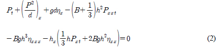
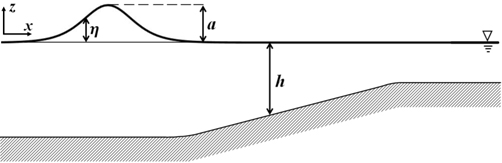
1차원 Madsen-Sørensen 확장형 Boussinesq 방정식(1992)을 지배 방정식으로 하며 아래의 식으로 표현된다(Madsen and Sørensen, 1992). Fig. 1은 시스템의 도식을 나타낸다.

Fig. 1

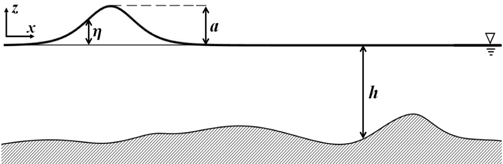
The schematic description of computational domain

위 식에서 η(x, t)는 수면변위, P(x, t)는 체적속도이며 h(x)는 정지수면에서의 수심, d( = h + η)는 전체 수심, g는 중력가속도, B는 조율계수(Calibration factor)이다. 아래 첨자 x와 t는 각각 ∂ / ∂x와 ∂ / ∂t를 의미한다. 본 연구에서 조율계수를 B = 1/15로 하여 지배방정식이 Stokes 1차 파랑 근사이론과 가장 유사한 값을 가지게 한다(Madsen and Sørensen, 1992).

지배방정식을 Crowhurst and Zhenquan(2013)가 제시하였던 유한차분, 수치 계산법을 도입하여 Kang et al.(2017)과 같은 방법으로 유한차분식을 도출한다(Crowhurst and Zhenquan, 2013; Kang et al., 2017).

위 유한차분식은 O(Δx)의 정도를 가진다. 아래 첨자 i와 위 첨자 n은 각각 공간축과 시간축의 교점 번호이고 Δx과 Δt은 각각 공간축과 시간축의 교점간격이다. 경계조건은 소멸조건으로하여 식 (5)와 식 (6)과 같이 나타내며, 초기조건은 일반적인 고립파를 나타내는 식을 사용하여 식 (7)과 식 (8)과 같이 한다 (Seabra-Santos et al., 1987; Kang et al., 2017).

위 식에서 N 은 시간교점의 최댓값, M + 1은 공간교점의 최댓값이다. 수심이 일정한 해저지형에서 격자를 변경시켜 가며 고립파 전파에 관한 수치 시뮬레이션을 실행하여 t = 10s일 때의 수치 결과와 엄밀해를 비교하여 오차(μ)가 O(10^-2)의 정도를 가지게 하는 격자 간격을 본 연구에서 사용한다. 오차는 아래의 식 (9)를 활용하여 구할 수 있다.

아래의 Table 1은 Δx와 Δt를 각각 변경했을 때의 오차를 나타낸다.

Table 1

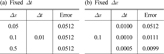
Error with regard to the size of mesh

수치 모델에서 공간 격자의 크기는 오차의 크기에 크게 영향을 미치지 않으므로 Δx = 0.1m로 하며, 시간격자의 크기는 오차의 정도가 O(10^-2)미만으로 하는 Δt = 0.0005s로 한다.

3. 수치 시뮬레이션

수치 시뮬레이션에서 격자의 크기는 Δx=0.1m, Δt=0.0005s이며 유한차분법의 수렴조건 (Courant–Friedrichs-Lewy condition, C_r)은 아래의 식을 이용하여 구할 수 있다(Lee and Cho, 2000; Kang et al., 2017).

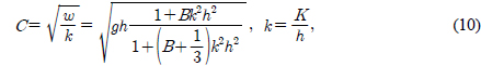
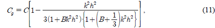
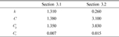
위 식들에서 k는 파수(Wave number), C는 위상 속도(Phase velocity), w는 각 주파수(Angular frequency), C_g 는 군속도(Group velocity)이다. 아래의 Table 2는 Δx = 0.1m, Δt = 0.0005s로 하였을 때, 3.1장, 3.2장에서 사용되는 수치 모델에서의 C_r 을 보여준다. 두 경우의 수치 모델에서 모두 C_r < 1을 만족시키는 것을 확인 할 수 있다.

Table 2

Courant–Friedrichs-Lewy conditions

3.1 완만한 경사의 해저 언덕 모델

Fig. 2와 같은 해저 언덕에서 경사가 각각 α₁ = 1/200과 α₂ = 1/400인 조건에서 수치 시뮬레이션을 하며, 해저 지형은 식 (13)과 같다(Klopman, 2010).

Fig. 2

The sketch of a mild slope

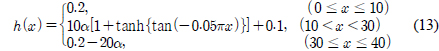
계산영역은 0m< x <40m(N = 400), 0s< t <22s(M = 44,000)이다. 10m< x <30m에 경사가 있으며, 초기 수심은 h₀ = 0.2m이며, 입사파의 위치와 진폭은 x₀ = 5m, a = 0.02m이다. 유효 파장은 L = 4.4m이며, 이는 고립파의 η/a = 0.01인 지점 사이의 거리이며 L = 21.86h₀로 구해진다(Wang and Liu, 2011).

비쇄파(Non-breaking) 파의 경우 군속도와 파의 에너지 밀도(E )의 곱 (G_gE)으로 나타나는 에너지 유동량(Energy flux)이 보존 된다. 진행파가 언덕을 만나기 전 일정한 수심을 지날 때는 일정한 속도와 형상을 유지하며 전파를 한다. 하지만 고정되어 있는 경사면을 지날 때 군속도는 감소되며, 이 감소된 양은 에너지 밀도의 증가로 보상되며 이로 인해 진폭이 증가하는 오름을 나타내게 된다(Wikipedia, 2016). 그 후, 진폭이 일정 높이에 다다르게 되면 더 이상 증가하지 않고 진행파가 분열하게 된다 (Madsen and Mei, 1969).

Fig. 3과 Fig. 4는 수치 시뮬레이션 결과와 Wang and Liu (2011)의 수치 결과를 나타내며, 두 결과가 잘 일치한다. t = 8s에 고립파가 경사에 도착하며, t = 15s에는 고립파가 경사를 지나고 있다. t = 22s에는 고립파가 경사를 완전히 통과한다. 고립파가 경사를 지날 때 오름 현상이 발생 하며 이 후, 고립파가 분열하여 작은 진폭의 고립파가 생긴다. 경사의 수평거리가 같을 때 경사의 기울기가 클수록 군속도의 감소폭이 더 커지므로 오름과 분열의 경향이 강하게 된다.

Fig. 3

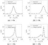
Comparison of the numerical results with those of Wang and Liu(2011) : α₁ = 1/200

Fig. 4

The numerical results compared to those of Wang and Liu(2011) : α₂ = 1/400

3.2 잠제 모델

Fig. 5 형태를 가지는 잠제 지형에서 고립파의 전파에 관한 수치 시뮬레이션을 실행 하며, 해저 지형은 식 (14)로 설정한다 (Klopman, 2010).

Fig. 5

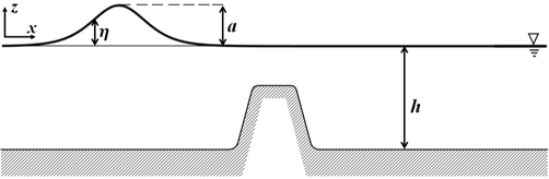
The computational domain of a submerged breakwater

수치 시뮬레이션의 계산영역은 −30m< x <20m(N = 500), 0s< t <8s(M = 16,000)이다. 입사파의 위치는 x₀ = −13m이며, 진폭을 a = 0.06m, a = 0.1m로 각각 설정한다. 잠제 이외의 지점에서의 수심은 초기 수심은 h₀ = 1m와 같다. 잠제는 x = 0m에 대하여 대칭의 형태를 가지고 있으며, 높이는 0.8m이다. 그리고 잠제의 왼쪽 면에서 기울기 γ = 1/2의 경사가 −2m< x <−0.4m에 존재한다. 고립파의 초기 진폭을 수치 시뮬레이션을 한다.

진행파가 경사를 만나기 전까지는 일정한 속도와 형상을 유지하며 전파를 하다가 고정되어 있는 잠제의 경사면을 지날 때 군속도는 감소되며, 이 감소된 양에 의해 에너지 밀도가 증가하게 되어 진폭이 증가하게 된다. 동시에 진행파가 잠제를 올라갈 때 경사의 영향으로 인해 반사파가 생긴다(Peregrine, 1967). 잠제의 정상을 지나 내려올 때는 군속도가 증가하여 진폭이 작아지게 된다. 하지만 반사파에 의한 에너지 손실로 인하여 초기 진폭보다 잠제를 완전히 통과했을 때의 진폭이 더 작게 된다 (Wikipedia, 2016).

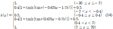
Fig. 6과 Fig. 7는 수치 시뮬레이션 결과와 Grilli et al.(1994)의 수치 결과를 나타낸다. 첫 번째 그래프는 고립파가 잠제에 도착했을 때의 형상이며, 두 번째 그래프는 최댓값의 진폭을 가질 때의 형상이며 오름 현상을 볼 수 있다. 나머지 두 그래프는 고립파가 잠제를 통과 한 후의 형상을 나타낸다. 두 진폭의 조건에서 두 결과들이 잘 일치하는 것을 확인 할 수 있다.

Fig. 6

Wave profiles compared to the conventional numerical data of Grilli et al.(1994) (a = 0.06m)

Fig. 7

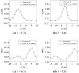
Computed wave profiles and the numerical data of Grilli et al.(1994) (a = 0.1m)

다음으로, 잠제의 기울기에 따른 파의 진폭 감소에 관한 수치 시뮬레이션을 한다. 초기 진폭을 a = 0.06m로 하고 Fig. 8처럼 잠제의 기울기를 γ₁ = 1/2, γ₂ = 1/4로 한다.

Fig. 8

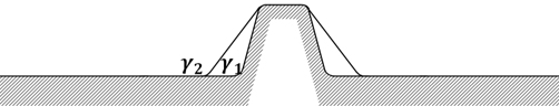
The geometry of the submerged breakwaters of different slopes

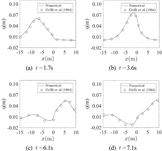
고립파의 파고가 무차원 공간 x′ = x/ h₀ = －6을 통과 할 때의 무차원 시간을 t′ = t( g / h₀)^0.5 = 0으로 하여, 진폭의 무차원 값인 η′ = η/h₀ 을 구하여 Ghadimi et al.(2016)의 수치 결과와 비교한 후, 기울기 변화에 따른 진폭 감소변화를 분석한다. Fig. 9는 고립파가 이동할 때 진폭의 크기를 나타낸다. Table 3은 각 기울기에서 t₁′ = 5.07, t₂′ = 12.99에서의 파의 위치와 그때의 평균 속도를 보여주며, Table 4은 t₂′ = 12.99에서의 무차원 진폭을 보여준다.

Fig. 9

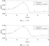
Values of amplitude with regard to x coordinate and the numerical data of Ghadimi et al.(2016) : γ₁ = 1/2, γ₂ = 1/4

Table 3

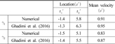
Mean velocity between t₁′and t₂′

Table 4

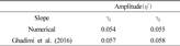
Solitary wave amplitude at t₂′ = 12.99

유체가 잠제를 통과하여 진폭이 작아지며, 동시에 유체의 속도가 증가하게 된다. 기울기가 더 클수록 잠제를 통과했을 때의 유체의 속도가 더 크며 운동에너지가 더 크다. 이로 인해 유체의 위치에너지 더 작게 되며 진폭이 더 작게 된다(Ghadimi et al., 2016).

4. 결 론

본 연구에서는 Crowhurst과 Zhenquan(2013)의 유한차분/수치 계산법을 활용하여 1차원 Madsen-Sørensen 확장형 Boussinesq 방정식(1992)을 두 가지 굴곡해저지형에서의 고립파에 대한 수치 시뮬레이션을 하였으며 해저지형에 의한 고립파의 여러 가지 물리적 변화를 확인 하였다.

(1) 완만한 경사의 해저 언덕에서 수치 시뮬레이션에서는 Wang과 Liu(2011)의 수치 결과와 잘 일치하는 것을 확인 할 수 있었다. 고립파가 경사에 도달하기 전에는 일정한 형상을 유지한 채 전파하였으며, 경사를 지나갈 때 군속도가 감소하고 에너지 밀도가 증가하여 진폭이 커지는 오름 현상을 확인 할 수 있었다. 그리고 진폭이 일정 높이에 다다르면 더 이상 증가하지 않고 진행파가 분열 되었다. 경사의 수평거리가 같을 때 경사의 기울기가 클수록 군속도의 감소폭이 커지므로 오름과 분열의 경향이 커지는 것을 확인 할 수 있었다.

(2) 잠제 지형에서 Grilli et al.(1994)의 수치 결과와 잘 일치하였다. 고립파가 경사에 도달하기 전에는 일정한 형상을 유지하였으며, 경사를 지나갈 때 진폭이 커지며 동시에 반사파가 발생하였다. 이 후, 잠제에서 내려올 때, 군속도가 증가하였으며 진폭이 감소하는 것을 볼 수 있었다. 하지만 반사파에 의한 에너지 손실로 인하여 초기 진폭보다 더 작아가 지는 것을 확인 할 수 있었다.

Ghadimi et al.(2016)의 수치 결과와의 비교를 통하여 파의 감소에 관한 잠제 기울기의 영향을 알아보았다. 잠제에서 내려 온 때 파는 진폭이 감소하며 유체의 속도가 증가하였다. 기울기가 더 클수록 잠제를 통과했을 때의 운동에너지가 더 크며, 이로 인해 위치에너지 더 작게 되어 진폭이 더 작게 되는 것을 확인할 수 있었다.

Article information Continued

References

Boussinesq, J., 1872. Théorie des ondes et des remous qui se propagent le long d'un canal rectangulaire horizontal, en communiquant au liquide contenu dans ce canal des vitesses sensiblement pareilles de la surface au fond. Journal de Mathématiques Pures et Appliquées, 2(17), 55-108.
Boussinesq J.. Théorie des ondes et des remous qui se propagent le long d'un canal rectangulaire horizontal, en communiquant au liquide contenu dans ce canal des vitesses sensiblement pareilles de la surface au fond. Journal de Mathématiques Pures et Appliquées 1872;2(17):55–108.Crowhurst, P., Zhenquan, L., 2013. Numerical Solutions of One-Dimensional Shallow Water Equations. UKSim 15th International Conference on IEEE, 55-60.
Crowhurst P., Zhenquan L.. Numerical Solutions of One-Dimensional Shallow Water Equations In : UKSim 15th International Conference on IEEE; 2013. p. 55–60.Ghadimi, P., Rahimzadeh, A., Chekab, M., 2016. Numerical Investigation of Free Surface Elevation and Celerity of Solitary Waves Passing over Submerged Trapezoidal Breakwaters. The International Journal of Multiphysics, 9(1), 61-74.
Ghadimi P., Rahimzadeh A., Chekab M.. Numerical Investigation of Free Surface Elevation and Celerity of Solitary Waves Passing over Submerged Trapezoidal Breakwaters. The International Journal of Multiphysics 2016;9(1):61–74.Grilli, S.T., Losada, M.A., Martin, F., 1994. Characteristics of Solitary Wave Breaking Induced by Breakwaters. Journal of Waterway, Port, Coastal, and Ocean Engineering, 120(1), 74-92.
Grilli S.T., Losada M.A., Martin F.. Characteristics of Solitary Wave Breaking Induced by Breakwaters. Journal of Waterway, Port, Coastal, and Ocean Engineering 1994;120(1):74–92. 10.1061/(ASCE)0733-950X(1994)120:1(74).Jang, T.S., 2017. A New Dispersion-Relation Preserving Method for Integrating the Classical Boussinesq Equation. Communications in Nonlinear Science Numerical Simulation, 43, 118-138.
Jang T.S.. A New Dispersion-Relation Preserving Method for Integrating the Classical Boussinesq Equation. Communications in Nonlinear Science Numerical Simulation 2017;43:118–138. 10.1016/j.cnsns.2016.06.025.Jang, T.S., 2018a. An improvement of convergence of a dispersion-relation preserving method for the classical Boussinesq equation. Communications in Nonlinear Science and Numerical Simulation, 56, 144-160.
Jang T.S.. An improvement of convergence of a dispersion-relation preserving method for the classical Boussinesq equation. Communications in Nonlinear Science and Numerical Simulation 2018a;56:144–160. 10.1016/j.cnsns.2017.07.024.Jang, T.S., 2018b. A new functional iterative algorithm for the regularized long-wave equation using an integral equation formalism. Journal of Scientific Computing, In press.
Jang T.S.. A new functional iterative algorithm for the regularized long-wave equation using an integral equation formalism. Journal of Scientific Computing 2018b;In press.Kang, S., Park, J., Jang, T.S., 2017. Numerical Simulation of 1D Shallow Water Waves Using Madsen-Sørensen Extended Boussinesq Equations on Slowly Varying Bottom. Proceedings of the Spring Conference of the Korea Ocean Engineering Society, Busan
. Kang S., Park J., Jang T.S.. Numerical Simulation of 1D Shallow Water Waves Using Madsen-Sørensen Extended Boussinesq Equations on Slowly Varying Bottom In : Proceedings of the Spring Conference of the Korea Ocean Engineering Society. Busan; 2017.Klopman, G., 2010. Variational Boussinesq Modelling of Surface Gravity Waves over Bathymetry. Doctoral dissertation, Wohrmann Print Service.
Klopman G.. Variational Boussinesq Modelling of Surface Gravity Waves over Bathymetry. Doctoral dissertation 2010. Wohrmann Print Service.Lee, C., Cho, Y.S., 2000. Extendability of Extended Boussinesq Equations : 1. Linear Dispersion Relation. Journal of Korean Society of Civil Engineering, 20(4B), 545-552.
Lee C., Cho Y.S.. Extendability of Extended Boussinesq Equations : 1. Linear Dispersion Relation. Journal of Korean Society of Civil Engineering 2000;20(4B):545–552.Madsen, O.S., Mei, C.C., 1969. The Transformation of a Solitary Wave over Uneven Bottom. Journal of Fluid Mechanics, 39(04), 781-791.
Madsen O.S., Mei C.C.. The Transformation of a Solitary Wave over Uneven Bottom. Journal of Fluid Mechanics 1969;39(04):781–791. 10.1017/S0022112069002461.Madsen, P.A., Sørensen, O.R., 1992. A New Form of the Boussinesq Equations with Improved Linear Dispersion Characteristics. Part 2. A Slowly Varing Bathymetry. Coastal Engineering, 18, 183-204.
Madsen P.A., Sørensen O.R.. A New Form of the Boussinesq Equations with Improved Linear Dispersion Characteristics. Part 2. A Slowly Varing Bathymetry. Coastal Engineering 1992;18:183–204. 10.1016/0378-3839(92)90019-Q.Peregrine, D.H., 1967. Long Waves on a Beach. Journal of Fluid Mechanics, 27, 815-827.
Peregrine D.H.. Long Waves on a Beach. Journal of Fluid Mechanics 1967;27:815–827. 10.1017/S0022112067002605.Seabra-Santos, F.J., Renouard, D.P., Temperville, A.M., 1987. Numerical and Experimental Study of the Transformation of a Solitary Wave over a Shelf or Isolated Obstacle. Journal of Fluid Mechanics, 176, 117-137.
Seabra-Santos F.J., Renouard D.P., Temperville A.M.. Numerical and Experimental Study of the Transformation of a Solitary Wave over a Shelf or Isolated Obstacle. Journal of Fluid Mechanics 1987;176:117–137. 10.1017/S0022112087000594.Wang, X., Liu, P.L.F., 2011. An Explicit Finite Difference Model for Simulating Weakly Nonlinear and Weakly Dispersive Waves over Slowly Varying Water Depth. Coastal Engineering, 58(2), 173-183.
Wang X., Liu P.L.F.. An Explicit Finite Difference Model for Simulating Weakly Nonlinear and Weakly Dispersive Waves over Slowly Varying Water Depth. Coastal Engineering 2011;58(2):173–183. 10.1016/j.coastaleng.2010.09.008.Wikipedia, 2016. Wave Shoaling. [Online] (Updated November 2016) Available at : https://en.wikipedia.org/wiki/Wave_shoaling/ [Accessed November 2016]
. Wave Shoaling 2016. [Online] (Updated November 2016) Available at : https://en.wikipedia.org/wiki/Wave_shoaling/. Accessed November 2016.