Various types of vortex flows occur in nature and engineering applications (Van Dyke, 1982; Lugt, 1983; Samimy et al., 2003). Helmholtz (1858) first investigated such vortex flows, and research on vortex rings, such as smoke rings, attracted attention from the beginning. In general, vortex rings are generated through the impulsive ejection of fluids. For example, vortex rings can be observed in jet flows for the propulsion of cephalopods (Krueger and Gharib, 2005).

Sir W. Thomson presented the translational velocity of the vortex ring of a small circular cross-section in the appendix of the paper written by Helmholtz (1867). Lamb (1932) verified the results obtained by Sir W. Thomson using the kinetic energy of the vortex ring. Fraenkel (1970) and Fraenkel (1972) analytically identified various physical occurrences of the small cross-sectional vortex rings through Fourier analysis. Spherical vortices were analyzed by Hill (1894).

Norbury (1973) investigated the general cases of the vortex rings including small cross-sections and the spherical vortex rings mentioned above, which are known as Norbury-Fraenkel family of vortex rings. Durst et al. (1981) determined the shape of a vortex ring by numerically solving partial differential equations for the stream function.

In this study, the Norbury-Fraenkel family of vortex rings is analyzed using a contour dynamics method (Shariff et al., 1989; Shariff et al., 2008). Stokes’ stream function was expressed as a contour integral using the Green’s function, and the integration of the logarithmic-singular segment, which occurs when the core shape is to be determined, was expressed analytically. The core shapes and the characteristic values of the vortex rings were compared with the results of previous studies to verify the validity of the proposed method.

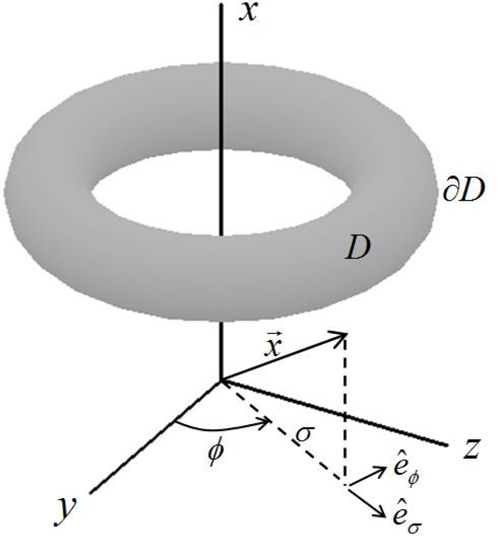
The fluid is assumed to be an ideal fluid. The flow is analyzed when the core of a vortex ring, in which the flow is rotational, exists in an irrotational infinite flow field, as shown in Fig. 1. The flow is axisymmetric with respect to the x-axis. If cylindrical polar coordinates are introduced in the analysis of the axisymmetric flow, as shown in the figure, the vorticity vector ω→→ is expressed as follows: where ω→→ is the flow velocity vector. The velocity vector of the axisymmetric flow is expressed as Stokes’ stream function ψ, as follows:

For an axisymmetric flow, the Helmholtz vorticity equation for a non-viscous incompressible fluid is expressed as follows (Batchelor, 1967):

From Eq. (3), the vorticity ω_ϕ is proportional to σ inside the core and is zero outside the core. where ∂D is the boundary of D, which is the inner core region, and Ω is a constant.

In considering the rotational flow of the incompressible fluid, the velocity vector is obtained by introducing the vector potential A→, as follows:

Eq. (6) is a gauge condition introduced to ensure the uniqueness of the solution. A→ is expressed using cylindrical polar coordinate components, as follows:

Based on Eq. (2) and Eqs. (5)–(7), the stream function ψ is expressed as follows:

In addition, substituting Eqs. (5) and (6) into Eq. (1) yields the Poisson equation for A→, as follows:

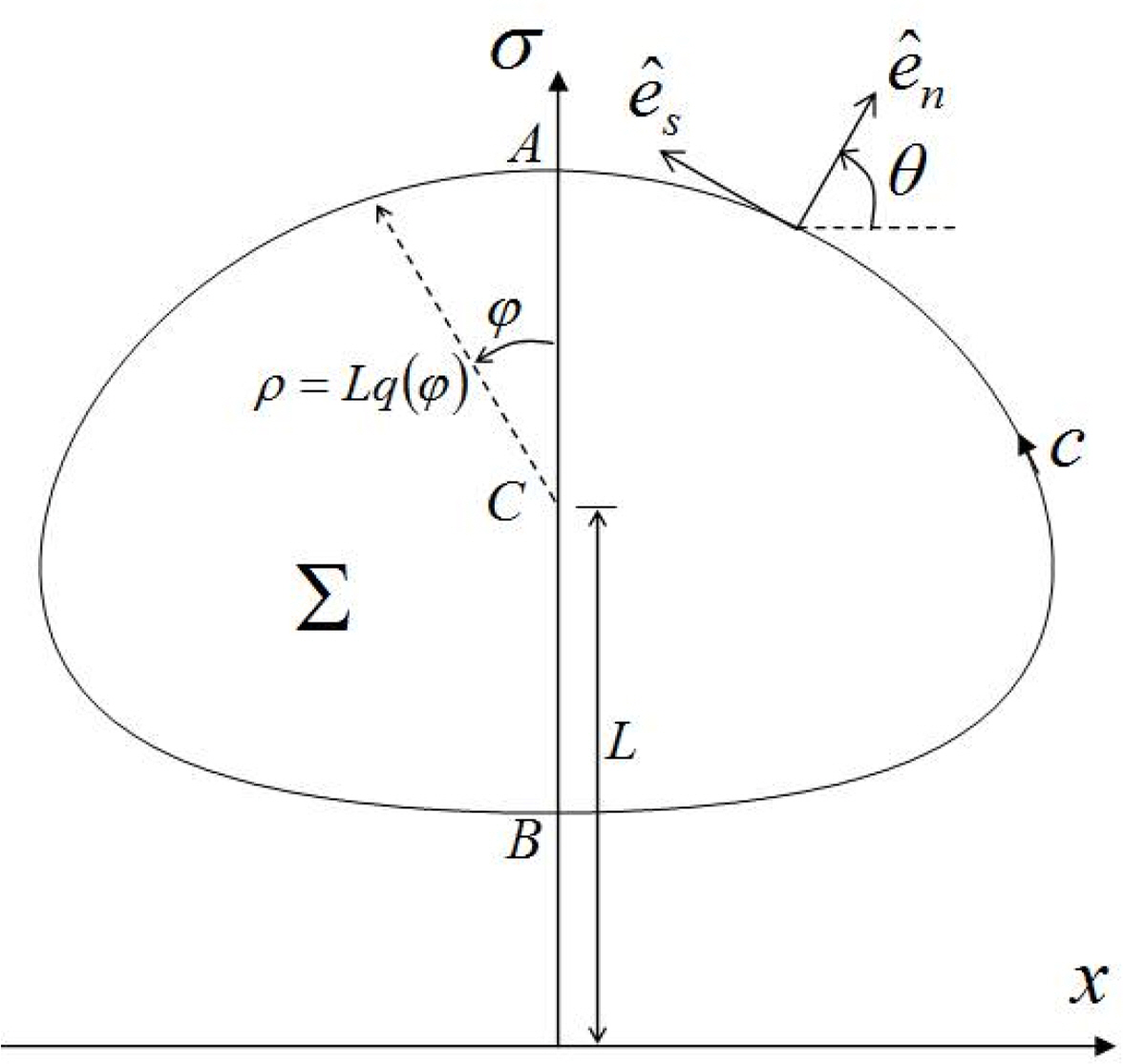
After A_ϕ is obtained by applying Green’s second identity to this equation, ψ is expressed, as shown in Eq. (10) using Eq. (8) (Fraenkel, 1970; Norbury, 1973). where Σ is the inner region of the core cross-section (Fig. 2). Additionally, K(k) and E(k) are the complete elliptic integrals of the first and second kinds (Gradshteyn and Ryzhik, 2000), and modulus k is defined as follows:

Shariff et al. (1989) and Shariff et al. (2008) obtained ψ as a contour integral using the vorticity jump (Eq. (4)) across ∂D . The results can be expressed as the following equations. where s, θ, and path c are defined in Fig. 2. The application of the contour dynamics method is beneficial in numerical calculations because it requires the one-dimensional integration on the contour instead of the two-dimensional integration of Eq. (10). In Eqs. (14) and (15), k→1 holds in the case of (x′,σ′)→(x,σ), and thus, G(s′) and H(s′) exhibit logarithmic singularity.

In this study, the Norbury-Fraenkel family of vortex rings, which are steady-state vortex rings, were the aim of the analysis. In this case, the vortex rings move forward at a steady-state velocity U in the positive x-direction. The free stream – Uê_x superposition used to express the flow velocity relative to the vortex rings leads to the expression of the stream function, as follows: where Ψ is the stream function in the coordinate system fixed to the vortex rings. As the flow cannot penetrate contour c, the stream function value must be a constant if the field point (x,σ) of Eq. (18) exists on contour c: where κ is a constant. Therefore, the contour shape can be determined if the field point (x,σ) that satisfies Eq. (19) is obtained.

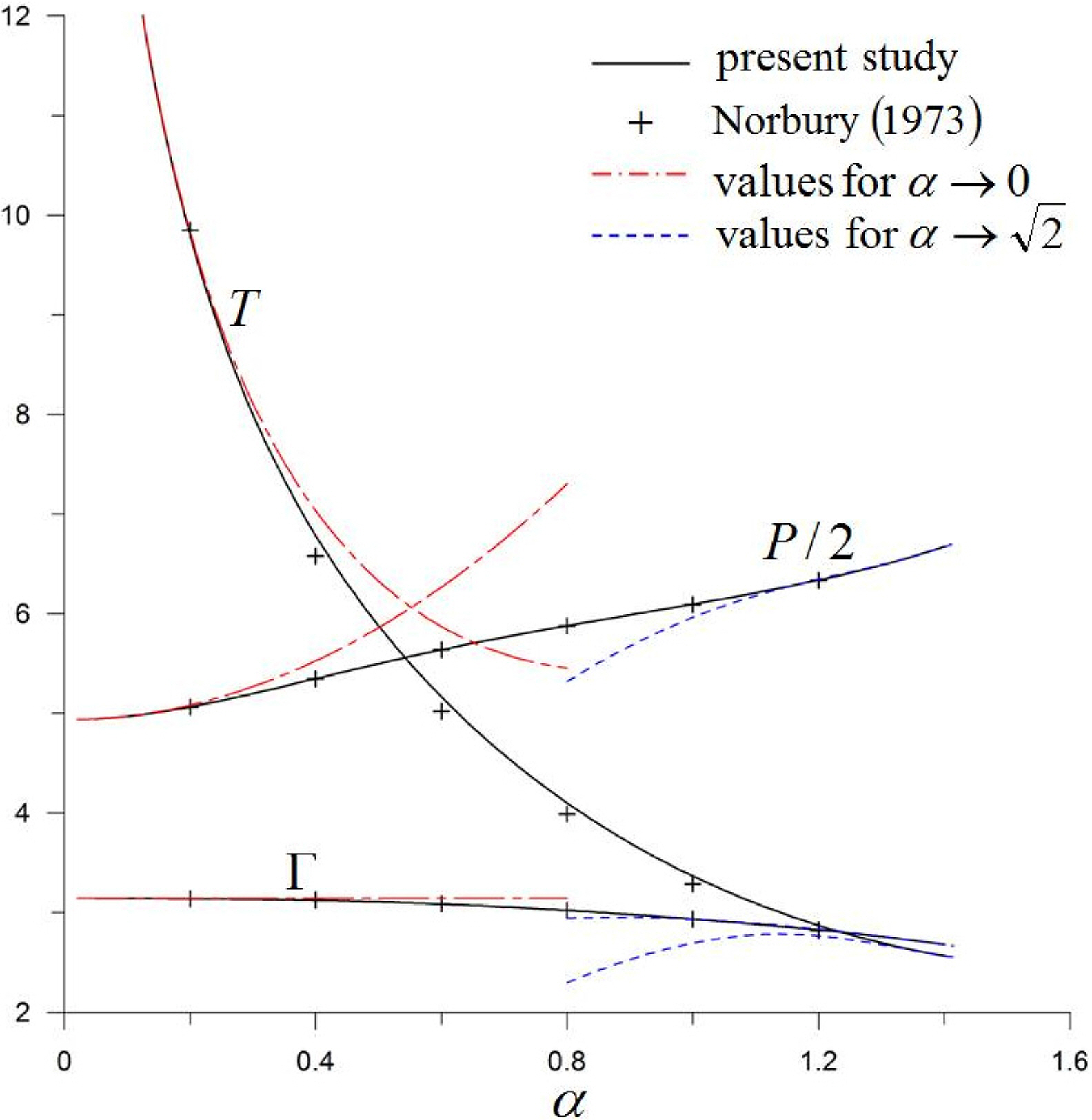
The circulation (Γ), vortical impulse (P), and kinetic energy (T) were evaluated as the physical properties of the vortex rings, as follows, to compare their values with those of previous studies. where ρ_f is the density of the fluid. Eqs. (21) and (22) are shown in Lamb (1932).

Norbury (1973) standardized the contour shape in non-dimensional form. In Fig. 2, the midpoint between Points A and B are defined as Point C, and the distance between the x-axis and Point C is defined as the ring radius L. Furthermore, the dimensionless mean core radius α defined by the following equation is introduced: where A_Σ is the area of the core cross-section. L is used to non-dimensionalize the geometrical quantities, as follows: where V_Σ is the volume of the core, and the symbol (∼) represents the non-dimensionalized physical quantity. Additionally, U, Ψ, κ, Γ, P, and T are non-dimensionalized, as follows:

In the following descriptions, the symbol (∼) is omitted in the expression of the non-dimensional quantities for convenience. Eqs. (12), (18), and (19) can be non-dimensionalized, as follows:

The parametric angle φ and the radial distance q(φ) from Point C are introduced to express the contour shape, as shown in Fig. 2.

The non-dimensionalized cross-sectional area and the characteristic values of the vortex rings are expressed as follows:

In Eq. (31), the range of the mean core radius α is 0<α≤2; in the case of α=2, it represents Hill’s spherical vortex (Batchelor, 1967). A contour integral was used in Eqs. (31)–(33), but a two-dimensional integration must be performed to obtain the kinetic energy of Eq. (34).

Fraenkel (1970) and Norbury (1973) determined the contour shape using the following two-dimensional integral equation that was used in Eq. (10). for (x,σ) on c

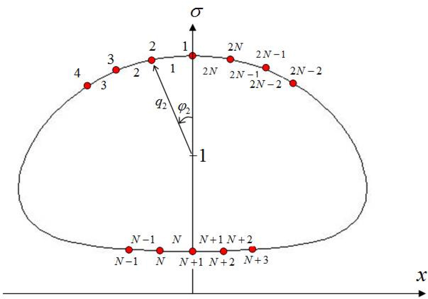
The contour shape is discretized as shown in Fig. 3, to numerically obtain the shape using Eq. (29). In this case, the number of nodal points and segments was set to 2N, considering the symmetry of the geometry.

The following relationships hold based on the definition of Point C (Fig. 2) and symmetry.

The discretized contour shape can be determined by obtaining q₁ ∼ q_N that satisfies Eq. (29) for the given α. In Eq. (29), κ and U are also the unknowns to be determined. Therefore, the total number of unknowns is N+2, and N+2 equations are, therefore, required to obtain the unknowns. N+1 equations are obtained by substituting N+1 field points (x_n, σ_n) corresponding to q₁ ∼ q_N into Eq. (29). If the condition of Eq. (31) is additionally assigned, N+2 nonlinear simultaneous equations are constructed. Broyden’s method, an iterative calculation scheme, is used to obtain the solutions of these equations (Press et al., 1992). In addition, the angle φ is divided into equal intervals.

In the iterative calculations, the numerical burden when the contour integral of Eq. (29) is used can be significantly reduced compared to the two-dimensional integration of Eq. (35), which was used by Norbury (1973).

The contour integral of Eq. (29) is obtained as the sum of segmental integrals, as follows: where (x_n,σ_n) is the field point, and c_i is the i-th segment. In this study, integration is performed by simplifying the segments into linear segments (Shariff et al., 1989; Shariff et al., 2008).

Substituting Eq. (40) into Eq. (39) yields the following expression.

When n ≠ i and n ≠ (i + 1), conventional numerical integration can be performed because the integrands of Eq. (41) exhibit non-singular behavior. In this study, numerical integration is performed using three-point Gauss-Legendre quadrature.

However, when n = i or n = (i + 1), the integration must be performed considering the logarithmic singularity that occurs at ξ = 0 or ξ = 1 respectively. For the case of n = i, Eq. (41) is expressed as follows:

In this study, H – G – 2J is asymptotically expanded in series form at ξ = 0 and analytically integrated based on the methods proposed by Shariff et al. (1989) and Shariff et al. (2008).

The integral values calculated by setting JM = 5 in Eq. (43) are presented in Appendix.

When δψ_n(x_{n + 1},σ_{n + 1}), it is possible that the signs of l_x and l_σ are reversed in Eq. (42), as well as in Eqs. (A1) and (A2) in Appendix. Then, the sign of the integral value is reversed after using σ_{n + 1} instead of σ_n

The appropriate selection of the initial guess is required to achieve the stable performance of the iterative calculation method. A circle with a radius of α was set as the initial guess contour for α ≤ 0.95, and a circle with a radius of 0.95 was used as the initial guess contour for 0.95 < α ≤ 1.1. In this case, 0.5 was used as the initial guess of κ and U . In the case of α > 1.1, the solutions for α = 1.1, 1.2, 1.3, and 1.39 were sequentially obtained and set as the initial guesses.

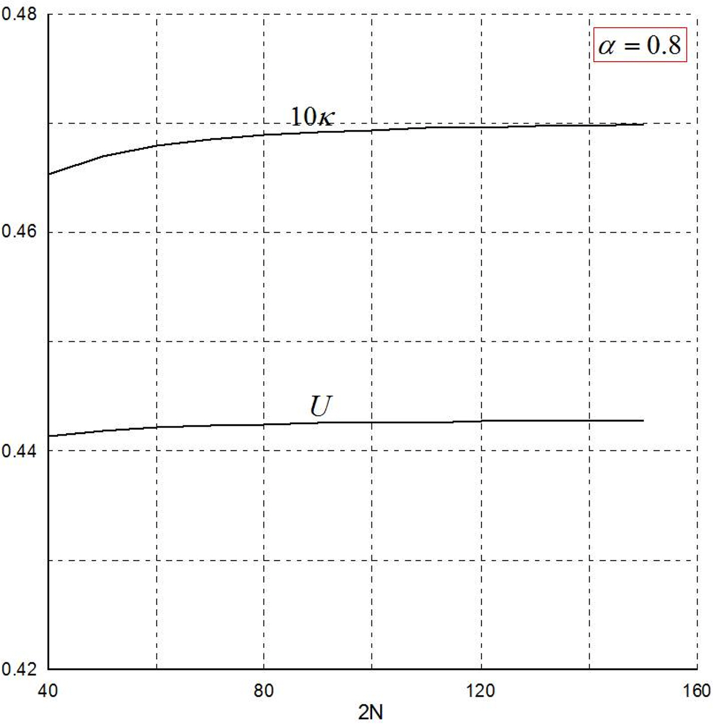
The convergence of the numerical solutions based on the number of segments was analyzed at α = 0.8. Fig. 4 shows the results of κ and the translational velocity U . As shown in Fig. 4, the solution is considered to have sufficiently converged if the number of segments, 2N, is approximately equal to 120. Therefore, for all the α values, calculations were performed using 2N = 120.

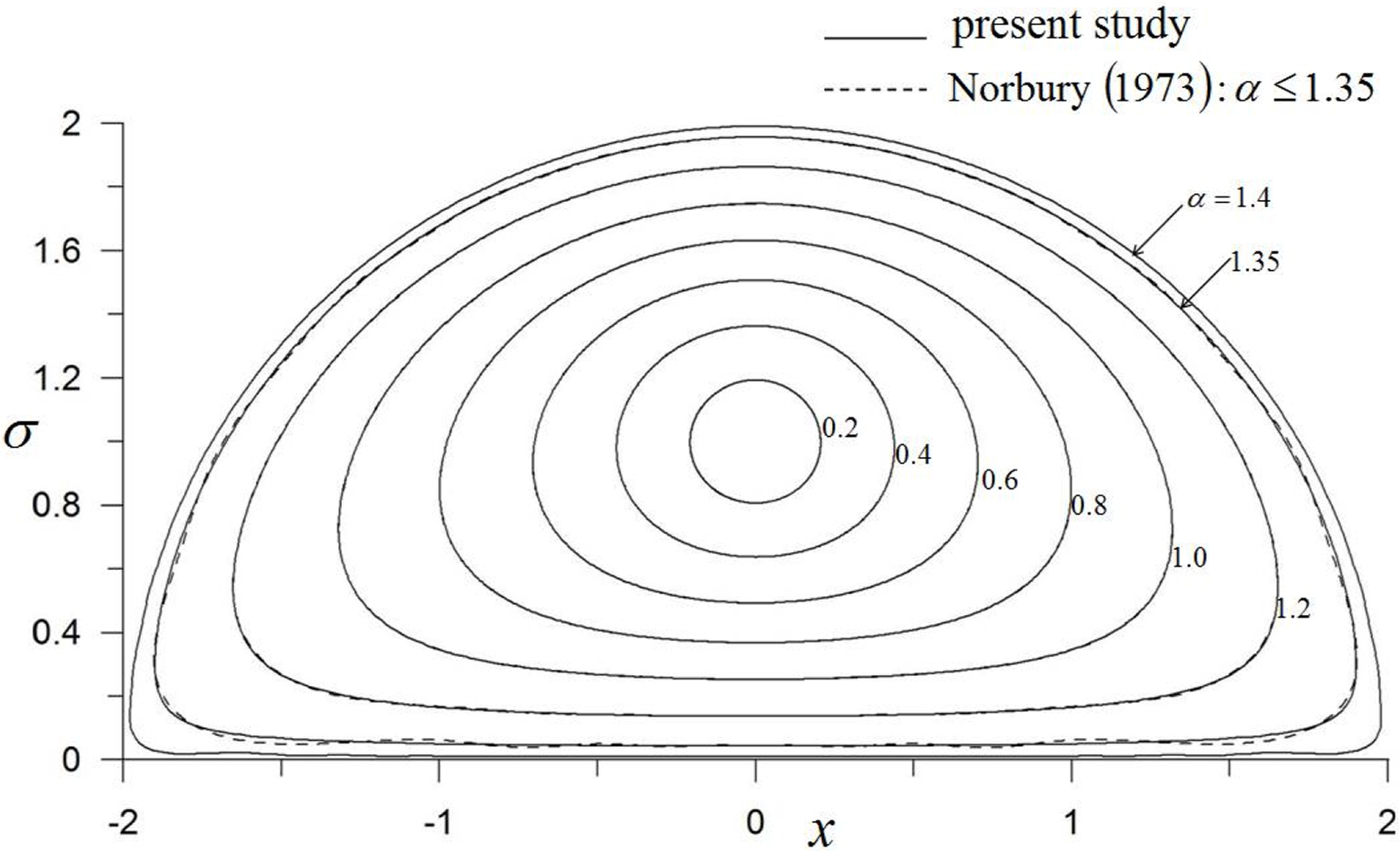
Fig. 5 shows the shapes of the cores for several α values. In Fig. 5, the results of Norbury (1973) are also displayed using dotted lines. Norbury (1973) used the two-dimensional integration of Eq. (35) and an indirect method to construct the core shape using Fourier coefficients that expressed the contour shape. The Fourier coefficients were obtained as the solutions of simultaneous equations. Although the technique applied by Norbury (1973) could be used to analyze the problem up to α = 1.35, in this study, it is possible up to α = 1.40, which is very closer to αmax=2≃1.414 (Hill’s spherical vortex). In addition, the numerical burden is significantly reduced by performing the contour integral instead of extensive calculations owing to the two-dimensional integration. In Fig. 5, the values between nodal points were interpolated through Fourier analysis of the decretized shape. The two results are almost identical when the value of α is small, but when the value is large, slight irregularities are observed in the results of Norbury (1973). This trend is due to the limited number of Fourier coefficients. In this study, however, this phenomenon was hardly observed because the positions of the nodal points were directly obtained.

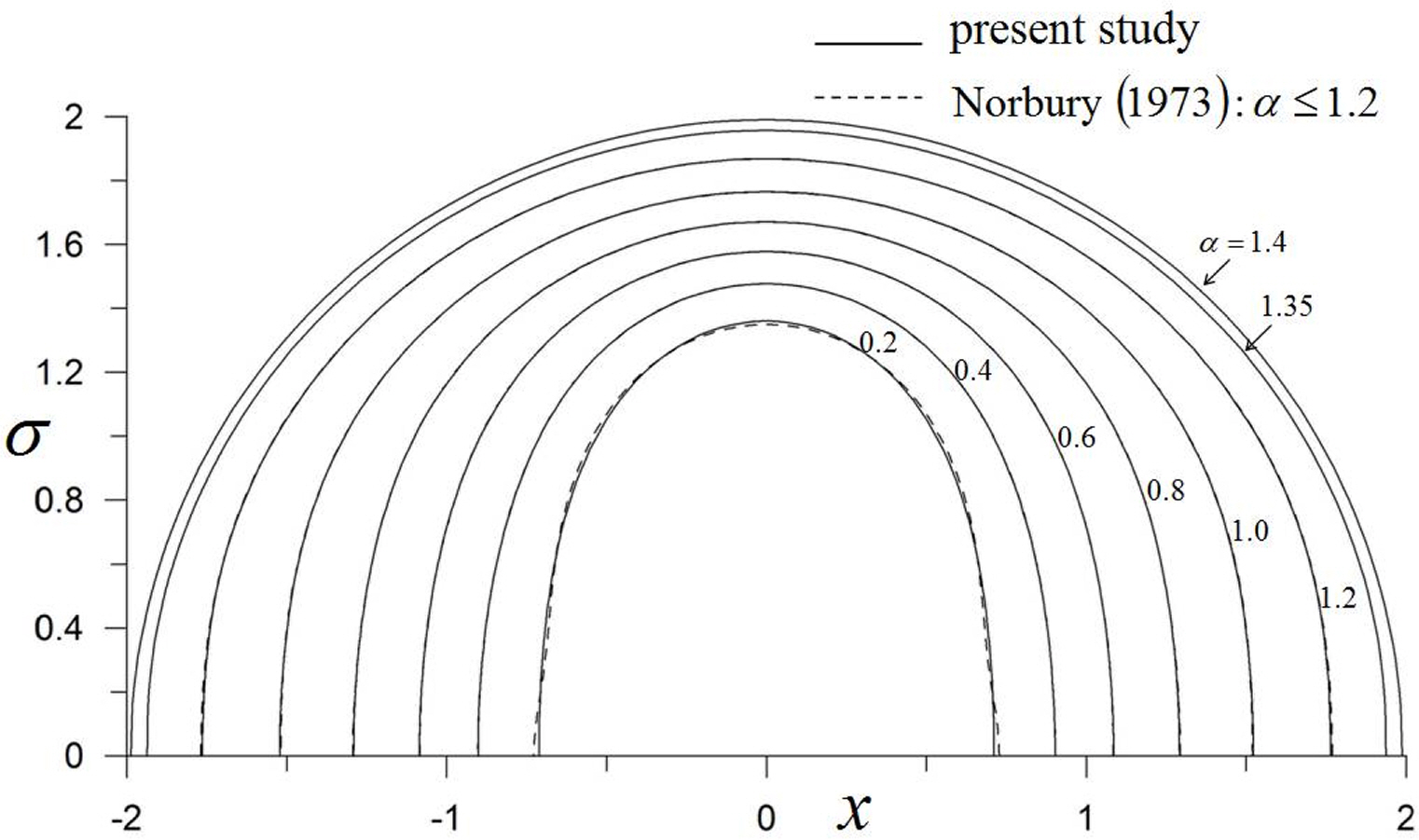
In a steady-state vortex ring, an irrotational flow region that moves forward at the same velocity with the ring exists. This region is known as the vortex atmosphere (Akhmetov, 2009). The shape of the vortex atmosphere is expressed by the dividing stream surface (Fig. 6) and can be obtained using the following equation.

The dividing stream surface was obtained for several α values, as shown in Fig. 7. As can be seen from Fig. 7, the results are in good agreement with those of Norbury (1973).

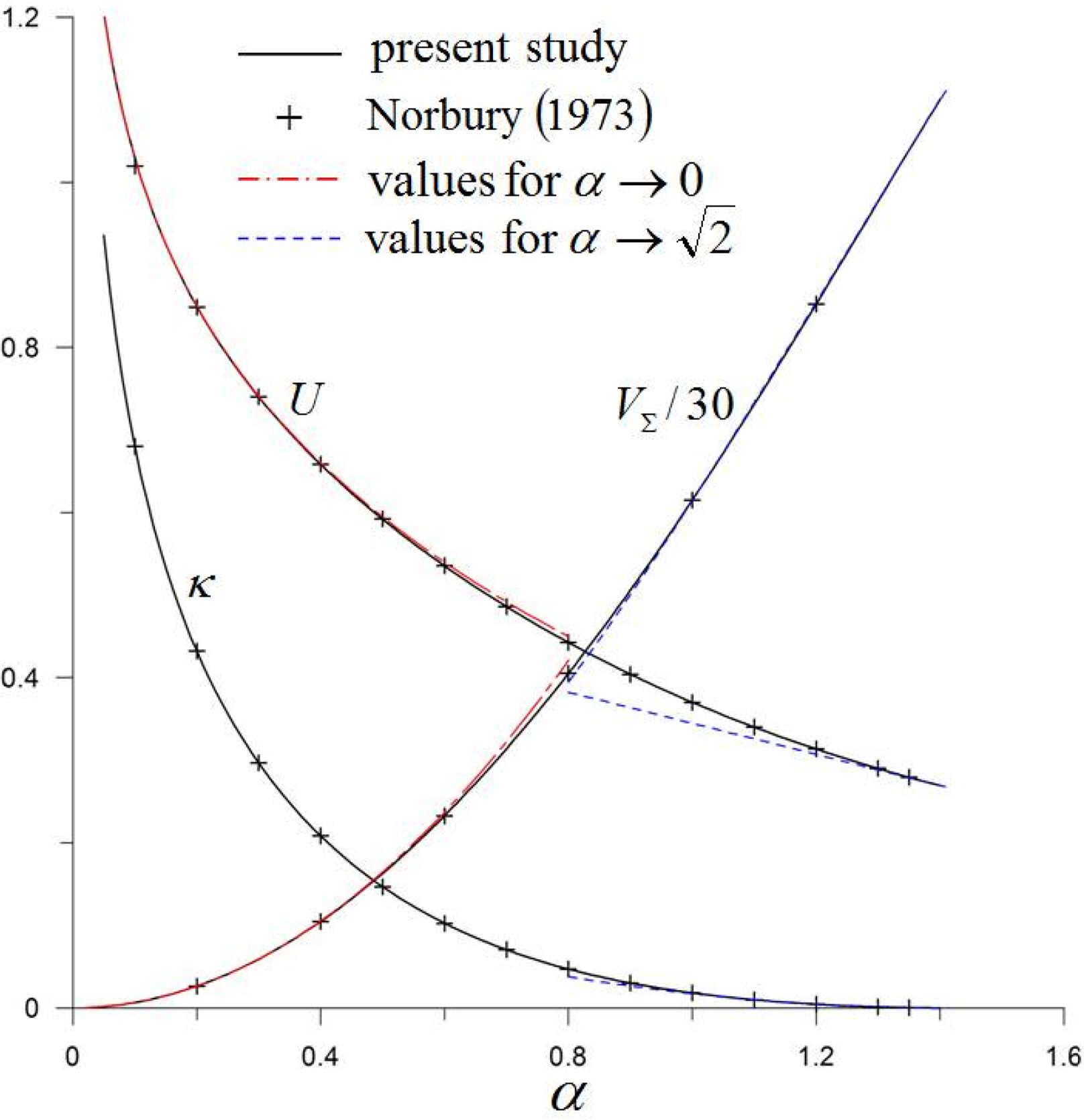
Fig. 8 shows the results for U, κ, and V_Σ. Those for small α values are as follows (Fraenkel, 1972):

Furthermore, asymptotic solutions for α→2 are as follows (Norbury, 1973):

As can be seen from Fig. 8, the results of this study are in good agreement with those of Norbury (1973). The results of this study are also in good agreement with the asymptotic solutions for α→0 and α→2, thereby validating the results of the proposed method.

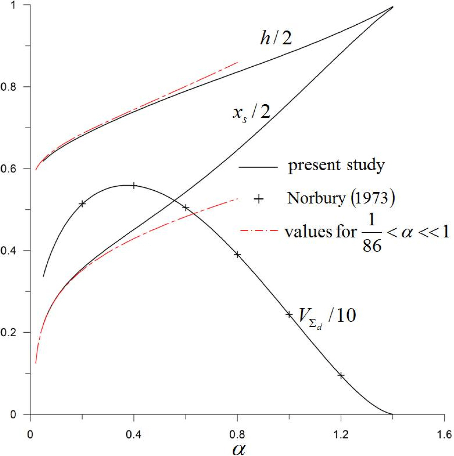
Fig. 9 shows the characteristic values of the dividing stream surface. The definitions of x_s and h are shown in Fig. 6, and V_Σd is the volume of Σ_d, which is an irrotational flow field in the vortex atmosphere. In the case of α > 1/86, the stagnation points exist on the x-axis (x =±x_s ), and the asymptotic solution of x_s for a small α value is expressed in Eq. (50) (Akhmetov, 2009). In addition, based on the model of Lamb (1932) for a small α value, h is expressed as the solution of Eq. (51).

The results of the dividing stream surface are also in good agreement with those of previous studies.

Fig. 10 shows the results of the circulation (Γ), vortical impulse (P), and kinetic energy (T). Based on the core volume (V_Σ), Γ can be obtained as follows:

The asymptotic solutions for α→0 and α→2 are as follows (Fraenkel, 1972; Norbury, 1973):

As can be seen from Fig. 10, the results for the circulation and vortical impulse are consistent with the findings of previous studies. The results for the kinetic energy are slightly higher than those of Norbury (1973), but they are in good agreement.

The Norbury-Fraenkel family of vortex rings was analyzed using a contour dynamics method for the Stokes‘ stream function. The calculation results for the core shape, dividing stream surface, and physical properties of the rings were compared with the findings of previous studies and asymptotic solutions to verify the validity of the proposed method.

The numerical burden was significantly reduced by performing the contour integral instead of a two-dimensional integration over the core cross-section. In addition, the difficulty of numerical integration was solved by analytically integrating over the logarithmic-singular segment. By directly determining the nodal point positions of the core shape, the results were better than those of the existing Fourier coefficients analysis method.

It is expected that the proposed method can also be applied to unsteady vortex ring problems if combined with the contour dynamics method for velocity.