
1. Introduction
Since Chappelear (1961) developed an early numerical method, many other numerical methods have been derived (Dean, 1965; Rienecker and Fenton, 1981; Chaplin, 1979; Cokelet, 1977; Fenton, 1988). Rienecker and Fenton (1981) solved the coefficients and some wave properties directly using NewtonŌĆÖs method. This method was further simplified by Fenton (1988). The major modification was that all the required partial differentials were calculated numerically (Tao et al., 2007). Although neither of the above numerical methods could be applied to waves in deep water (Fenton, 1990), Shin (2023) calculated deep water breaking waves with an error of less than 2.04├Ś10ŌłÆ3 percent, demonstrating that Fourier approximation is effective even for deep water waves. The objective of this study was to extend ShinŌĆÖs method (Shin, 2023) to include rotational water waves with a shear current in a finite depth (Shin, 2022). The basic concept of ShinŌĆÖs method (Shin, 2023) for establishing a set of equations was similar to FendonŌĆÖs method (Rienecker and Fenton, 1981; Fenton, 1988), and some issues with FentonŌĆÖs method have been addressed. The first issue is inherent in NewtonŌĆÖs method, which necessitates an initial solution in close proximity to the final solution. In common with other versions of the Fourier approximation method (Chappelear, 1961; Dean, 1965; Chaplin, 1979), it is sometimes necessary to solve a sequence of lower waves, extrapolating forward in height steps until the desired height is reached (Fenton, 1988). These methods can occasionally converge to the wrong solution with very long waves (Fenton, 1988). This paper shows that regression analysis can easily avoid this issue (Shin, 2019).
The second issue arises from the coordinate system. Because FentonŌĆÖs method adopts the moving coordinate system proposed by Dean (1965), the abscissa is the position from the crest in the range, ŌłÆLŌēżxŌēżL. Therefore, the relative position with respect to the wavelength, L, is unknown because the wavelength is unknown. As a result, the number of unknown variables to be determined in FentonŌĆÖs method is more than double the number in this study. Furthermore, a nonlinear equation for calculating the wavelength was coupled to the set of equations for calculating the coefficients. This coupling complicates the problem because NewtonŌĆÖs method requires partial derivatives with respect to the wavelength. The issue can be avoided easily using the dimensionless coordinate system in Fig. 1 because it is independent of the wavelength. The abscissa is the phase in the range ŌłÆŽĆŌēż╬▓ŌēżŽĆ, and is known. After determining the steepness, S, the wave-number is calculated as k=S/H because wave height, H is known. The steepness is calculated using the wave height condition, which is integrated automatically into the set of equations because it is linear. Therefore, it is not necessary to calculate the partial derivatives with regard to the wavelength in this study.
The third issue arises from the water depth condition used to calculate the reference depth, D, which is unknown. FentonŌĆÖs method requires partial derivatives with respect to the reference depth because the water depth condition is coupled to the set of nonlinear equations used to calculate the coefficients. Most errors in FentonŌĆÖs method occur when the water depth condition is calculated numerically. The required series order must be increased to reduce the error, and SimpsonŌĆÖs rule was used for the numerical integration. This issue was avoided by calculating the reference depth independently using the shooting method in the study. In numerical analysis, the shooting method is used to solve a boundary value problem by transforming it into an initial value problem. A set of ŌĆ£nŌĆØ equations with ŌĆ£nŌĆØ unknowns can be converted to a set of ŌĆ£nŌłÆ1ŌĆØ equations with ŌĆ£nŌłÆ1ŌĆØ unknowns because one variable can be calculated independently, assuming it is a known value in advance. The assumed value was determined using the shooting method. Although it has the disadvantage of requiring the calculation of one procedure as two procedures, the numerical formulation simplifies the process and significantly reduces the total number of steps needed to converge to a complete solution. The reference depth is not coupled to the set of equations for calculating the Fourier coefficients because the water depth condition is calculated independently.
The fourth issue is a method for calculating the partial derivatives required in NewtonŌĆÖs method. While all the necessary partial derivatives were obtained numerically in Fenton (1988), they were calculated analytically by tensor analysis in the present study. Therefore, there are no errors in the partial derivatives in this study.
Although the above-mentioned studies are irrational flows, this study is rotational flow based on Shin (2022). The numerical method used to calculate the Fourier coefficients and the related wave properties was not presented by Shin (2022) but is presented in the present study. Shin (2018) presented the numerical method for irrotational waves. The method was extended to rotational waves in this study. Shin (2022) reported the complete solutions to the Euler equations and calculated the waves by Le Mehaute et al. (1968). The fluid velocities calculated by irrotational wave theories (Fenton, 1990; Tao et al., 2007) and by rotational wave theory (Shin, 2022) were compared with the experimental data reported by Le Mehaute et al. (1968) on the same graphs. Unlike the irrotational waves, the results of the rotational wave theory agreed well with the experimental data. The calculated wave-breaking limit was in good accordance with the Miche formula. While Rienecker and Fenton (1981), Fenton (1988), Tao et al. (2007), Cokelet (1977), and Vadden-Broeck and Schwarts (1979) calculated the dispersion relations for some waves in a relative depth of 0.7, this study calculated these relations for many waves with different heights at various depths. The results were then extrapolated to all waves using regression analysis (Shin, 2019). The dispersion relations for a relative depth of 0.7 were compared and showed good accordance with the other results. The convergence of this study was tested according to the series orders. Even for relatively small orders, the error was significantly lower than FentonŌĆÖs method and Tao et al. (2007).
2. The Complete Solution to the Euler Equations
This chapter summarizes the solution reported by Shin (2022). The two coordinate systems were adopted. The first was a conventional coordinate system (t, x, y), as reported by Dean et al. (1984), in which the origin is located at a fixed point on the still water line (SWL). The x-axis is in the direction of wave propagation; the y-axis points vertically upward, and t is the time. The fluid domain is bounded by a flat bed, y = ŌłÆh (water depth), and by a free surface y = ╬Ę (t, x). The second is a dimensionless coordinate system, (╬▓ ╬▒), as shown in Fig. 1, which is a stationary frame. The origin is located under the crest of the bed. Therefore, the wave profile is fixed with a periodic, even function in the system. The abscissa is phase ╬▓ = kx ŌłÆ Žēt in ŌłÆŽĆ Ōēż ╬▓ Ōēż ŽĆ, where k = 2ŽĆ/L is the wave number and Žē = 2ŽĆ/T is the angular frequency. Here, T is the wave period; L is the wavelength, and the ordinate is the dimensionless elevation from the bed, ╬▒ = k(y + h) in 0 Ōēż ╬▒ Ōēż ╬│, where ╬│ = k(╬Ę + h) is the dimensionless free surface elevation from the bed. The term ╬Č = ╬│ ŌłÆ D is a dimensionless free surface elevation measured from the reference line (the horizontal line passing through two points on the free surface at two phases ╬▓ = ┬▒ŽĆ/2. The reference depth D = k(╬Ęo + h) is the dimensionless distance from the bed to the reference line where ╬Ęo = ╬Ę(┬▒ŽĆ/2). Because the coordinate system is independent of the wavelength, it has several advantages, as presented by Shin (2023). The dimensionless quantity of a flow field f is denoted by f╠ä except for those defined separately, such as S and ╬Ė. Using the notation, the stream function is defined by Žł = Žł╠äŽē/k2.The horizontal and vertical velocities are defined by u = Cu╠ä and v = Cv╠ä, respectively, where C = Žē/k is the celerity. The vorticity is defined by ╬® = Žē╬®╠ä. The pressure is defined by p = ŽüC2p╠ä, where Žü is the water density. The dimensionless wave height (steepness) is defined by S = kH. The linear steepness ╬Ė = Žē2H/g (where g is the gravity) is a constant for a particular wave. When h ŌåÆ Ōł× and H ŌåÆ 0, S ŌåÆ ╬Ė, which gives the dispersion relation (Žē2 = gk) of deep water linear waves. The stream function to satisfy the incompressible Euler equations is as follows:
where
Ōī® n Ōī¬ def ╠│ n 2 + ╬Ą
This solution also contains irrotational waves, where the constant, ╬Ą is referred to as the strength of vorticity because ╬®╠ä = 0 when ╬Ą = 0. When ╬Ą is non-positive, the vorticity has the same direction as the motion of the particles. The iso-stream and iso-vorticity lines can be calculated using NewtonŌĆÖs method in the Appendix. The free surface is an iso-vorticity line given by ╬®╠ä(╬▓,╬│) = C1╬Ą, where C1 is a constant. Substituting ╬®╠ä(╬▓,╬│) = C1╬Ą into Eq. (2), the wave profile is determined to satisfy the KFSBC (Kinematic free surface boundary condition) as follows:
The constant C1 is determined from the definition of the reference line in Fig. 1; that is, ╬│(┬▒ŽĆ/2) = D. The profile is an implicit function that can be calculated using NewtonŌĆÖs method in the Appendix. When ╬Ą ŌåÆ 0, Eq. (3) yields the profile defined by Shin (2018). Moreover, the sea bed is an iso-vorticity line given by ╬®╠ä(╬▓,0) = 0. Differentiating Eq. (1) with respect to ╬▒ and ╬▓, the horizontal velocity becomes the following.
Substituting Eqs. (1)ŌĆō(5) to the Euler momentum equations, BernoulliŌĆÖs principle for rotational flow can be calculated as follows.
where U╠ä2 = V╠ä2 ŌłÆ ╬Ą (╬▒ ŌłÆ Žł╠ä)2, and Q is a constant. A mechanical analog to irrotational and rotational flows was depicted by considering a carnival Ferris wheel in Fig. 2.11 in Dean et al. (1984). While the irrotational motion of chairs involves rotating around the center of the Ferris wheel, the rotational motion of the chairs involves both revolving around the center of the Ferris wheel and rotating around their center. Therefore, the total kinetic energy of the rotational motion is represented by the sum of the revolving kinetic energy around the center of the Ferris wheel and the rotating kinetic energy around their center. Analogous to the Ferris wheel, the total kinetic energy of rotational flow is represented by U╠ä2 = V╠ä2 ŌłÆ ╬Ą (╬▒ ŌłÆ Žł╠ä)2, where the first term corresponds to the revolving kinetic energy around the center of the Ferris wheel, and the second term corresponds to the rotating kinetic energy around its center. When ╬Ą = 0, U╠ä2 = V╠ä2 = (1 ŌłÆ u╠ä)2 + v╠ä2, which is the kinetic energy for irrotational flow. In contrast to Baddour et al. (1998), ╬Ą is not positive because kinetic energy functions should be positive-definite functions. Therefore, let
╬Ą def ╠│ ŌłÆ Žā 2 ╬ø 0 n ( ╬▓ , ╬▒ ) def ╠│ c 0 cos n ╬▓ cosh Ōī® n Ōī¬ D { Ōī® n Ōī¬ cosh Ōī® 0 Ōī¬ ╬▒ cosh Ōī® n Ōī¬ ╬▒ ŌłÆ Ōī® 0 Ōī¬ sinh Ōī® 0 Ōī¬ ╬▒ sinh Ōī® n Ōī¬ ╬▒ } ╬ø n m ( ╬▓ , ╬▒ ) def ╠│ Z 1 cosh ( Ōī® n Ōī¬ + Ōī® m Ōī¬ ) ╬▒ cos ( n ŌłÆ m ) ╬▓ + Z 2 cosh ( Ōī® n Ōī¬ ŌłÆ Ōī® m Ōī¬ ) ╬▒ cos ( n ŌłÆ m ) ╬▓ + Z 3 cosh ( Ōī® n Ōī¬ + Ōī® m Ōī¬ ) ╬▒ cos ( n + m ) ╬▓ + Z 4 cosh ( Ōī® n Ōī¬ ŌłÆ Ōī® m Ōī¬ ) ╬▒ cos ( n + m ) ╬▓ Z 4 = Ōī® n Ōī¬ Ōī® m Ōī¬ + n m + ╬Ą 4 W
(8)
(9)
For the average speed Ūs over a wave period on still water, the strength of vorticity is as follows:
From StokesŌĆÖ breaking criterion, |U╠äb| Ōēż 1 and |U╠äs| Ōēż 1. The BernoulliŌĆÖs constant Q is determined from the definition of the reference line (i.e., ╬│(ŽĆ/2) = D) and the DFSBC (Dynamic free surface boundary condition), i.e., p╠ä(ŽĆ/2, D) = 0 because the point (ŽĆ/2, D) is on the free surface. Therefore, the pressure field is
By applying the DFSBC, i.e., p̄(β, γ) = 0 on α = γ to Eq. (12), the other wave profile can be determined as follows:
3. NewtonŌĆÖs Method for Coefficients and Steepness
The solution contains N+2 unknown constants: N Fourier coefficients, cn, steepness, S, and reference depth, D. Eqs. (3) and (13) present two wave profiles with implicit functions. The two wave profiles are even functions considering the coordinate system. The Fourier series of a periodic even function is presented as
f ( x ) = Ōłæ n = 0 Ōł× c n cos n x Ōłæ n = 0 N c n cos n x m = f ( x m )
Referring to Eqs (3)ŌĆō(5), the denominators are expressed as transcendental functions of the reference depth. When determining the reference depth using NewtonŌĆÖs method in conjunction with the coefficients, it is necessary to calculate the partial derivative with respect to the reference depth. Furthermore, Eq. (15) only permits a numerical approach. This difficulty can be overcome by calculating the reference depth independently using the shooting method, assuming that the reference depth is known. Based on the assumption, Eq. (15) is independent of the other equations and will be calculated in the next chapter. In addition to this assumption, N parameters, Xm, are introduced in this chapter to simplify the numerical formulation. Unlike FentonŌĆÖs method, Xm are merely parameters for calculating the coefficients and the steepness in this chapter. After determining the coefficients, Xm are no longer used. Hence, the wave elevation is denoted with Xm instead of ╬Čm in this chapter.
When the wave profile ╬Č and the reference depth D are prescribed, it is possible to convert Eq. (3) into a set of linear equations for the coefficients. Because the wave profile is an even function, the phases ╬▓m(m = 1,2, ŌĆ”, N) are considered in the range 0 Ōēż ╬▓m Ōēż ŽĆ and ╬▓m ŌēĀ ŽĆ/2 because the two wave profiles are already equal at phase ╬▓ = ŽĆ/2. In addition, ╬▓1 = 0 and ╬▓N = ŽĆ. Denoting ╬Č(╬▓m) as Xm, i.e., Xm = ╬Č(╬▓m), Eq. (3) is presented.
The summation convention is considered in Eq. (16). The repeated subscript ŌĆ£nŌĆØ is a dummy subscript, whereas Kmn is a second-order tensor, and the terms cn and Xm are vectors in N-dimensional space. From Eq. (3), the component of the tensor Kmn is presented as
where X╠äm = Xm + D. Because Ōī®0Ōī¬= Žāi, the component of the first-order tensor, Ym is presented as
The summation convention is not applied when the component of a tensor is presented as in Eqs. (17) and (18). Using the inverse tensor Gmn of the tensor Kmn, the solution to Eq. (16) is determined easily as follows.
Eq. (13) is also evaluated at the same phase. A set of N nonlinear equations for calculating the N parameters Xn is obtained by substituting Eq. (19) into Eq. (13) at the same phase because the wave height condition in Eq. (14) is expressed as S = X1 ŌłÆ XN in this approach. For NewtonŌĆÖs method, the error vector Em is defined from Eq. (13) as follows:
Substituting Eq. (19) into Eq. (20)Ep = 0 gives a set of nonlinear equations for calculating the parameters, Xq. Therefore, unlike FentonŌĆÖs method (Rienecker and Fenton, 1981; Fenton, 1988), the set of N nonlinear equations is solved using NewtonŌĆÖs method in this study. Therefore, when using the same series order, the number of unknown constants is less than half of that in FentonŌĆÖs method.
Denoting partial derivatives of a tensor by making use of commas and indices as
Ōłé ( ) Ōłé X q = ( ) , q
The superscript (r) means the step of NewtonŌĆÖs method. It is clear that all the steps are rth in all equations except Eq. (24). Thus, for the simplification of equations, the superscript (r) was omitted in all the equations except Eq. (24). Differentiating Eq. (20) with respect to Xq, the partial derivative Ep,q of the error vector is
Note that cn,qcm = cncm,q Because S = X1 ŌłÆXN,
Differentiating Eq. (16) with respect to Xp results in
Multiplying Eq. (27) by the tensor Gim, the partial derivative of the coefficient is determined as follows.
where GimKmn = ╬┤in and ╬┤incn,p = ci,p and ╬┤in is the second-order isotropic tensor. Differentiating Eq. (17) with respect to Xp, the components of the third-order tensor Kmn,p are presented as
Differentiating Eq. (18) with respect to Xp, the component of the second-order tensor Ym,p is presented as
Differentiating Eq. (21) with respect to Xq, the component of the third-order tensor Apn,q is expressed as follows:
Differentiating Eq. (22) with respect to Xq, the component of the forth-order tensor Bpnm,q is
B p n m , q = ╬┤ p q [ Z 1 * sinh ( Ōī® n Ōī¬ + Ōī® m Ōī¬ ) X ┬» p cos ( n ŌłÆ m ) ╬▓ p + Z 2 * sinh ( Ōī® n Ōī¬ ŌłÆ Ōī® m Ōī¬ ) X ┬» p cos ( n ŌłÆ m ) ╬▓ p + Z 3 * sinh ( Ōī® n Ōī¬ + Ōī® m Ōī¬ ) X ┬» p cos ( n + m ) ╬▓ p + Z 4 * sinh ( Ōī® n Ōī¬ ŌłÆ Ōī® m Ōī¬ ) X ┬» p cos ( n + m ) ╬▓ p ] . Z 1 * = Z 1 ( Ōī® n Ōī¬ + Ōī® m Ōī¬ ) Z 2 * = Z 2 ( Ōī® n Ōī¬ ŌłÆ Ōī® m Ōī¬ ) Z 3 * = Z 3 ( Ōī® n Ōī¬ + Ōī® m Ōī¬ ) Z 4 * = Z 4 ( Ōī® n Ōī¬ ŌłÆ Ōī® m Ōī¬ )
(32)
Based on the assumption that the reference depth is known, Eq. (16) is linear and decoupled from Eq. (20), unlike in FentonŌĆÖs method (Rienecker and Fenton, 1981; Fenton, 1988). Dividing the inner product of the error vector, Em by N, the mean squared error (MSE) in the DFSBC is defined as
The MSE is used as a criterion for determining the convergence of the Newton method.
Shin (2019) was used as the first step,
X m ( 0 )
The profile satisfies the definition of the reference depth, i.e., ╬Č(┬▒ŽĆ/2) = 0, the wave height condition in Eq. (14), and the water depth condition in Eq. (15). Replacing ╬Č with
X m ( 0 )
4. Shooting Method for Reference Depth
In contrast to the assumption considered in Ch. 3, the reference depth is closely linked to the coefficients and is unknown. Therefore, while maintaining the validity of the method presented in Ch. 3, the shooting method is suitable for determining the reference depth. The reference depth is adjusted until the calculated water depth from the water depth condition matches the actual value using the shooting method. The secant method is used as a root-finding algorithm. In each step of the secant method, substituting the calculated coefficients and the prescribed reference depth into Eqs. (A1)ŌĆō(A4), the wave elevations
╬Č i ( q )
The reference depth is calculated using the secant method as follows.
where
where D(0) is determined using the regression result in Shin (2019), and h is the actual water depth. The actual value is in the vicinity of D(0). Hence, D(1) is selected with a value close to D(0), e.g., D(1) = 1.001D(0). For each step, the error in the water depth is as follows:
5. Calculation Procedure and Results
5.1 Calculation Procedure
Fig. 2 presents a flowchart. While there is only one do-loop in FentonŌĆÖs method, the chart comprises three do-loops. The outer do-loop implements the secant method for calculating the reference depth, as described in Ch. 4. The first inner do-loop implements the Newton method for calculating the coefficients and steepness, as described in Ch. 3. The other inner do-loop implements NewtonŌĆÖs method for calculating the wave profile, as described in the Appendix.
Initial approximations of the shape factor, steepness, and reference depth are first calculated by substituting the period, height, and depth into the regression analysis results presented by Shin (2019). The initial approximations of the wave profile are calculated using Eq. (34).
The first inner do-loop is performed. The coefficients,
c n ( r , q ) c n ( r , q ) Δ X i ( r , q ) X i ( r + 1 , q ) X i ( r , q ) X i ( r + 1 , q )
The second inner do-loop is then performed to calculate the free surface elevations at more phases than those considered in the first inner do-loop. The elevations,
╬Č i ( r + 1 , q )
By substituting
╬Č i ( q ) ( : l i m r ŌåÆ Ōł× ╬Č i ( r + 1 , q ) ) X m ( 0 , q + 1 ) X m ( Ōł× , q ) def ╠│ lim r ŌåÆ Ōł× X m ( r , q ) X m ( 0 , q + 1 ) = X m ( Ōł× , q )
5.2 Application Range of this Study
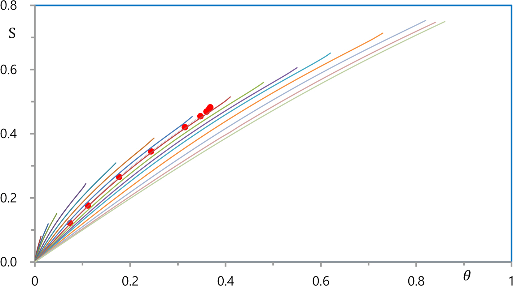
The coefficients and wave properties are functions of two variables: the reference depth and the linear steepness. The functions are presented with closed-form solutions in Shin (2019), which are the regression results determined using numerically calculated data for 2091 waves, as shown below. The domain of the functions is {(╬Ė, D) | 0 Ōēż ╬Ė < 1 and 0 < D}. A subset of the domain, {(╬Ė, D) | 0 Ōēż ╬Ė < 1 and 0 < D < 5}, was considered instead of the entire domain because waves are similar to deep water waves when D > 5. Seventeen cases of the reference depth were considered by dividing the domain by D = 0.1, 0.15, 0.2, ..., 1.0, 1.2, 1.5, 2, 3, 4, and 5. For each reference depth, the linear steepness was considered from 0 to 0.98 at 0.01 intervals, from 0.98 to 0.989 at 0.001 intervals, from 0.989 to 0.9899 at 0.0001 intervals, and from 0.9899 to 0.98997 at 0.00001 intervals, resulting in 123 cases of linear steepness. Therefore, 17 ├Ś 123 = 2091 irrotational waves were calculated with N = 35 and M = 180. The limits can be determined easily because the Newton method presented in the Appendix diverges at the crest when the steepness reaches its limit. These limits were represented by 17 red solid circle symbols in Fig. 3, which are calculated with D = 0.1, 0.15, 0.2, ..., 1.0, 1.2, 1.5, 2, 3, 4, and 5 in sequence from left to right. The solid curve is the regression analysis result determined using the 17 data. As shown in Fig. 3, the breaking limit is in good accordance with the Miche formula. Because the 2091 waves are dimensionless waves, they represent all waves below the breaking limit. Therefore, this study confirms stable convergence characteristics for all water waves.
5.3 Water Particle Velocities Under the Crest
The eight waves considered in Le M├®haut├® et al. (1968) were calculated. Fig. 3 and Table 1 present the waves with solid diamond symbols. The results were compared with experimental data in Fig. 2 by Shin (2022). Fig. 4 shows the wave (h) during the eight waves. Referring to Fig. 2 of Shin (2022), the other waves give the same pattern, as shown in Fig. 4. The irrotational results were calculated with ╬Ą = 0. The regression analysis results were calculated by Shin (2019).
Rienecker and Fenton (1981) also calculated the waves, as shown in Fig. 2 of that work. The waves were also calculated by Fenton (1990), and the results are shown in Fig. 3(c) of that work. The cnoidal theory is the new cnoidal theory by Fenton (1990), which closely agrees with the Fourier approximation by Fenton (1988). Tao et al. (2001) also calculated the waves; the results are shown in Fig. 2 of that work. HAM (Homotopy analysis method) by Tao et al. (2001) results closely agree with the Fourier approximation reported by Rienceker et al. (1981). Therefore, the Fourier approximation and HAM results are not presented in Fig. 4. This study agrees with the experimental data, unlike those obtained using HAM or FentonŌĆÖs method.
5.4 Dispersion Relation
Table 3, of Tao et al. (2007) provides a detailed comparison of the HAM solutions of waves in finite water depth and the results of Cokelet (1977) and Rienecker and Fenton (1981). The results are given in terms of the non-dimensional phase speed squared kC2/g at various values of H/h, for a constant value of exp(ŌłÆkR/C) = 0.5 (R is the unit span denoting the total volume rate of flow underneath the steady wave per unit length in a direction normal to the x, z plane), corresponding to a wavelength to water depth ratio of L/h Ōēł 9 (Tao et al., 2007). Table 1 of Rienecker and Fenton (1981) presents the same comparison between the solutions of Rienecker and Fenton (1981) for N = 16, 32, and 64, the results of Cokelet (1977), and the results of Vanden-Broeck & Schwarts.
The non-dimensional phase kC2/g is presented with physical quantities defined in this study as follows:
H/h is also presented with physical quantities defined in this study.
kh = 2ŽĆ/9 in Eq. (41) because L/h Ōēł 9. Therefore, the comparison shows the relationship between steepness, S, and linear steepness, ╬Ė for the relative water depth, kh = 2ŽĆ/9. Hence, the comparison shows the dispersion relation of waves in a finite water depth, kh = 2ŽĆ/9. Table 2 lists the relation. The data in the first and second columns were cited from Rienecker and Fenton (1981), which are the results calculated using N = 64. The data in the fourth column was obtained by multiplying the data in the second column by 2ŽĆ/9, as stated in Eq. (41). The data in the third column was obtained by multiplying the data in the first column by the data in the fourth column, as stated in Eq. (40). Shin (2018, 2019) also calculated the relation for various water depths, D = 0.1, 0.15, 0.2, ... , 1.0, 1.2, 1.5, 2, and Ōł×. For a given reference depth, the linear steepness ╬Ė was considered with a highly dense interval from 0 to the application limit of this study. Fig. 5 presents the calculation results. The 15 curves are the results calculated with D = 0.1, 0.15, 0.2, ... , 1.0, 1.2, 1.5, 2, and Ōł× in sequence from left to right. The peaks of each curve represent the limit of wave breaking. The nine data in Table 2 are also presented with solid circles in Fig. 5, which agree with the curve for D = 0.7. The small difference results from the difference between kh = 2ŽĆ/9 and D = 0.7. The relative depth for D = 0.7, is presented as kh = D ŌłÆ k╬Ę0 = 0.7 ŌłÆ k╬Ę0 > 2ŽĆ/9. because D = kh + k╬Ę0 and k╬Ę0 is negative. Therefore, the D = 0.7 curve lies slightly to the right of the eight data because k╬Ę0 is very small.
5.5 Error Check of this Study
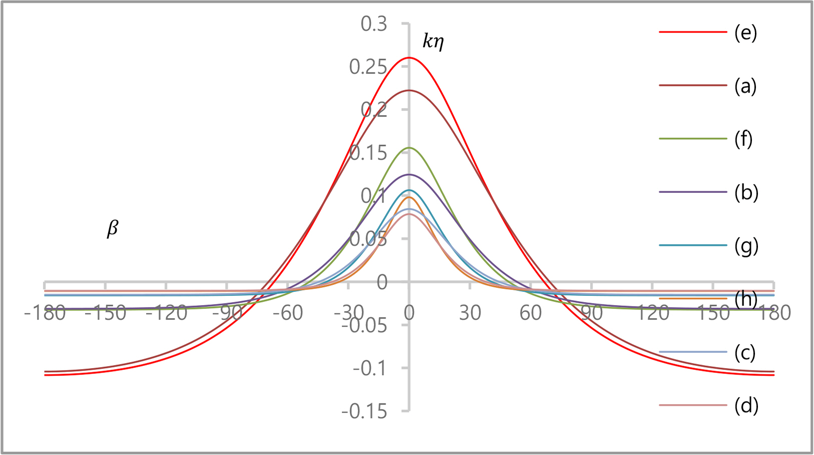
The numerical method focuses on minimizing the errors in the DFSBC defined in Eq. (20) and the water depth conditions defined in Eq. (15). The convergence of this study according to the series order was analyzed by calculating the eight waves considered in Le M├®haut├® et al. (1968) using N = 8, 10, 16, and 35. Fig. 6 presents the calculated wave profiles for the waves. The abscissa represents the phase ╬▓ = kx ŌłÆ Žēt in ŌłÆ180┬░ Ōēż ╬▓ Ōēż 180┬░, while the ordinate represents the dimensionless elevation, k╬Ę. The errors are summarized in Tables 3, and 4,. The first step is the result of Shin (2019). Table 3, lists the error of Shin (2019). There are three steps for calculating the water depth condition using the secant method and three steps for the Newton method at each secant step. Therefore, there are 10 steps; Table 4, presents the errors for step 10. The blanks indicate that they are unsuitable. The series order, N = 8, is unsuitable for waves (c) and (d), and the series order, N = 10, is unsuitable for wave (d) because they do not satisfy the condition for regular waves. Hence, there is no local extrema between the crest and the trough in a regular wave. The deeper the water depth and the lower the wave height, the smaller the number of series orders required. If the series order is increased beyond the optimal number, the convergence of this study decreases, as presented by Shin (2023). Even for very long waves, the convergence is very stable, unlike other methods.
6. Conclusions
This paper reported a numerical method to calculate the Fourier coefficient, steepness, and reference depth parameter. The method is much simpler than FentonŌĆÖs method or HAM. The partial derivatives with respect to wavelength and reference depth, as well as certain parameters, were eliminated utilizing a dimensionless coordinate system. The water depth condition was calculated independently using the shooting method in this study.