
1. Introduction
Waves are a complex phenomenon that occurs in the ocean or coastal areas owing to environmental variables, such as winds, and they play an important role in various marine and maritime fields. Particularly, safety at sea, maritime transportation, stability of marine structures, and marine ecosystems are directly affected by waves. According to the marine accident statistics from 2018 to 2022 provided by the Ministry of Oceans and Fisheries, wave-related accidents accounted for 21% of the total marine accidents (Ministry of Oceans and Fisheries, 2023). Therefore, accurate wave predictions are essential for ensuring the safety of navigating ships and marine operations at new locations, managing resources, and producing energy.
Previously used wave prediction methods include numerical modeling methods and statistical modeling methods. The numerical modeling methods for predicting waves simulate the motions of wave patterns using mathematical models. These methods have evolved through various models, such as the Sea Wave Modeling Project (SWAMP) (SWAMP Group, 1985), the Shallow Water Intercomparison of Wave Model (SWIM) (Group et al., 1985), the Wave Model (WAM) (Group, 1988), and the Wave Watch III (WW3) (Tolman, 2009). Carter (1982) used the Joint North Sea Wave Project (JONSWAP) method to predict wave height and wave period, and You and Park (2010) utilized a regional wave prediction system (Regional Wave Watch III, RWW3), which replaces the WAM model, to analyze the characteristics of the waves in the waters around Korea. In particular, Son and Do (2021) calibrated and optimized the third-generation Simulation Waves Nearshore (SWAN) model, which predicts waves using the wind field. These models utilize mathematical equations to represent the physical process of wave generation. The numerical methods have a high accuracy because they consider various factors, such as wind, water depth, current speed, and current direction. However, these methods require complex computations and substantial computing time, which lead to considerable costs. On the other hand, the statistical modeling methods use statistical techniques to predict waves. Furthermore, these methods analyze past wave data to discern patterns and trends and predict future waves. As the statistical modeling methods have lower computational complexity than the numerical methods, they have faster execution times. However, they have lower accuracy because they cannot consistently predict irregular and nonlinear waves. Kang et al. (2016) employed the autoregressive integrated moving average (ARIMA) model among the statistical models to predict significant wave heights in the East Sea of Korea. In addition, Adytia et al. (2018) applied the wind data provided by the European Centre for Medium-range Weather Forecasts (ECMWF) to the ARIMA model to predict wind and waves in the coastal area of Jakarta. Moreover, machine learning specialized for processing nonlinear data was proposed to overcome the limitations of the numerical and statistical modeling methods, and wave predictions have been performed based on this approach.
Machine learning has advanced over the past decade, and it can be applicable for predictive analyses in all fields, including revenue prediction, market price forecast, health prediction, and wave prediction (Masini et al., 2023). Predictions of marine environmental variables are performed by training machine learning models on data collected from marine observation equipment. Kumar et al. (2018) used an extreme learning machine to predict wave heights in the waters of Mexico, Brazil, and Korea. Domala et al. (2022) employed machine learning methods, including random forest, XGBoost, gradient boosting, and FBProphet, to predict waves in the North Atlantic Ocean and the coastal waters of Puerto Rico and Hawaii. They also presented optimal algorithms. Hu et al. (2021) used the XGBoost and long short-term memory (LSTM) methods to predict waves in Lake Erie, North America. Kim et al. (2022) developed the STG-OceanWaveNet model based on deep learning and used it to predict waves for a 48-h period based on the significant wave height, mean wave period and direction, and wind data. Machine learning methods, such as random forest and XGBoost, do not reflect the temporal dependency of the data and do not capture the sequential nature of the data. Consequently, they have low prediction accuracy. On the contrary, recurrent neural networks (RNNs) have been designed to use sequential or time-series data. As opposed to conventional feedforward neural networks, in which information moves from the input layer to the output layer in one direction only, RNNs have recursive connections that enable them to retain information from previous inputs.
This study employs RNN, LSTM, and gated recurrent unit (GRU) models, which have RNNs. Unlike previous studies that utilized the wind field data, this study additionally utilizes wave data from previous time periods to improve the accuracy of wave predictions. Furthermore, data from multiple observation points in the sea are integrated, rather than a single observation point, to minimize spatial constraints. The models are evaluated using the data from each observation point. Furthermore, to assess the performance of the models, the prediction results are compared with the results of the algorithms optimized for each observation point. The suggested wave prediction model by sea area can ensure the safety of marine and maritime operations and the efficient management of resources at new locations. In addition, as data provided by the Korea Hydrographic and Oceanographic Agency (KHOA) can be used without processing them, it is expected that real-time wave predictions will be performed through online learning in the future.
2. Prediction Model
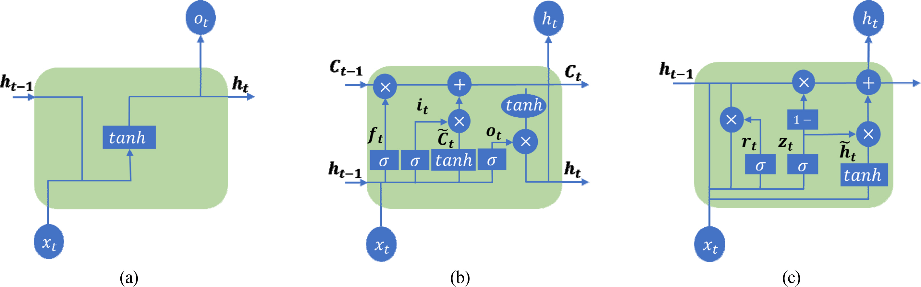
This study introduces the RNN, LSTM, and GRU deep learning models suitable for processing time-series data, and the structure of each model is illustrated in Fig. 1. Fig. 1(a) shows the structure of an RNN, which is specialized for processing sequential data, such as time-series data. The input to this neural network consists of the present and the past, and it has a hidden state. In addition, information is passed to itself at each step of the network (Pushpam and Enigo, 2020). Here, the input of the current time and the hidden state of the previous time are considered. Moreover, Wh denotes the weight matrix used to update the hidden state, and bh denotes the bias of the hidden state. tanh is a hyperbolic tangent activation function, which limits input values to a range between −1 and 1. RNNs calculate the hidden state of the current time ht by combining the current input xt and the hidden state of the previous time ht−1. ht is then passed on to the next time step to maintain continuous information. However, the vanishing gradient and exploding gradient problems occur in RNNs, depending on the values of the weights. To solve these problems, Hochreiter and Schmidhuber (1997) introduced a gate mechanism and proposed an LSTM, which learns data with long-term dependencies more effectively than RNNs. However, the LSTM had several limitations, including the absence of the forget gate, complexity, and computational cost. Gers et al. (2000) proposed an improved version of LSTM that has been used to date. Fig. 1(b) shows the structure of an LSTM, which consists of a forget gate, an input gate, an output gate, and an update cell state. This structure is an enhanced version compared with that of RNNs. The forget gate determines whether to preserve or delete the information from the cell state of the previous time, and the output is calculated by combining the current input and the hidden state of the previous time. The input gate plays the role of determining how much to update the cell state at the current time step, and it consists of the output of the input gate and a candidate for the cell state. The cell state adds the current input to the past information to represent the overall state at the current time. The output gate plays the role of determining the hidden state based on the cell state at the current time, and it is composed of two main elements: the output of the output gate and the determination of the hidden state at the current time. Finally, in the determination of the hidden state, the hidden state at the current time is determined by performing an element-wise multiplication of the output of the output gate and the cell state at the current time via tanh. LSTMs have three gates and a cell state. Hence, they have the drawback of having a complex structure, which increases the training time and computational complexity. Furthermore, there is a risk of overfitting if the amount of data is small. To address these issues of LSTMs, Chung et al. (2014) proposed the GRU, which only has a reset gate, an update gate, and a hidden state. Fig. 1(c) shows the structure of a GRU, which consists of two gates and a hidden state. The reset gate plays the role of determining whether the information from the previous hidden state will be reflected in the calculation of the current hidden state, whereas the update gate determines which information from the previous hidden state will be retained and which information from the previous hidden state will be replaced with the new hidden state. The candidate hidden state is determined by combining the current input with the previous hidden state adjusted by the reset gate. Finally, the GRU determines the final hidden state by performing an element-wise multiplication of the update gate result from the previous hidden state and the update gate result from the candidate hidden state and adding them.
Eqs. (1)–(3) represent the process of calculating the learning parameters for each model using mathematical expressions. Here, ninput denotes the number of input units that are fed into the model, and nhidden denotes the number of hidden state units for the model. The number of learning parameters for all the models is calculated by combining ninput and nhidden, and this number varies according to the structure of the model. Comparing Eq. (2) with Eq. (3), it is observed that a GRU, a simplified structure of an LSTM, has 25% fewer learning parameters than the LSTM and is computationally more efficient.
3. Experimental Data Setup
3.1 Dataset and Analysis
The data used in this study were the oceanographic buoy data from the KHOA. Fig. 2 shows the locations of the oceanographic buoys.
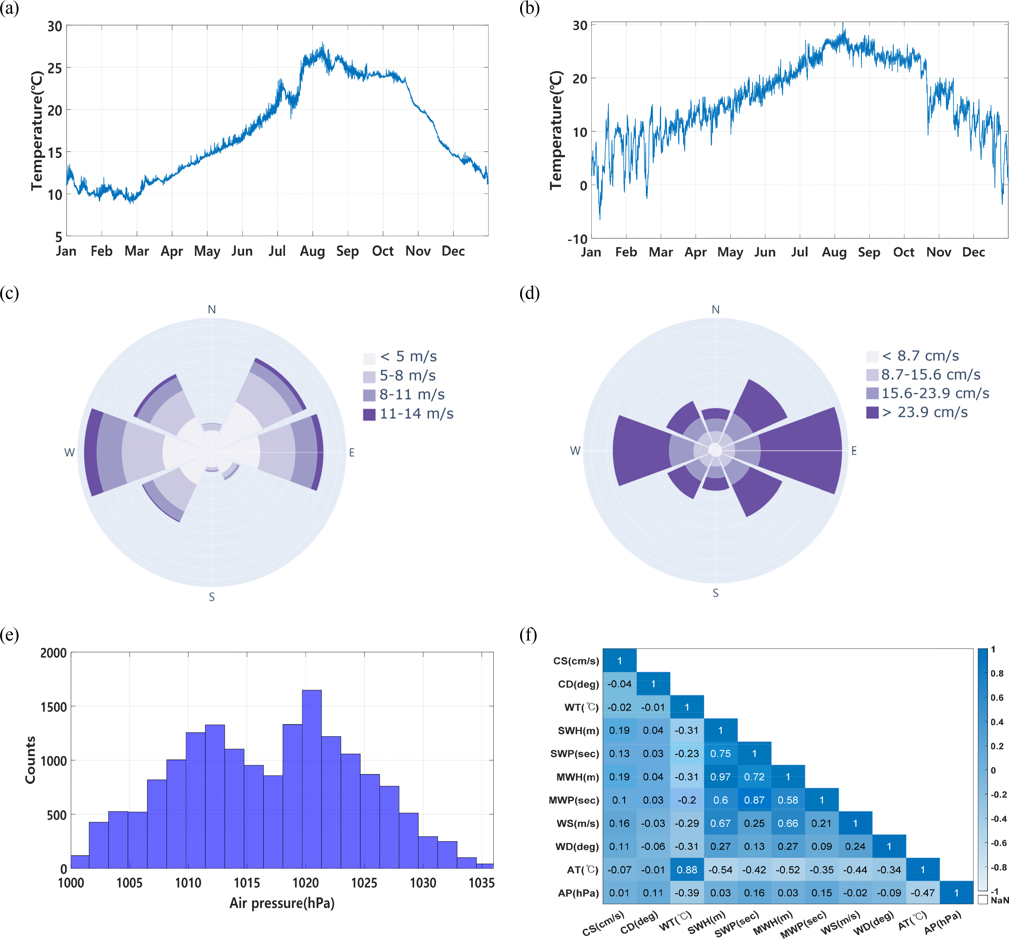
The observation points in the East Sea include four locations besides Gyeongpodae Beach, and three locations excluding Ulleungdo are beaches. In the South Sea, there are five locations besides Haeundae Beach. Moreover, in both the Jeju Coastal Sea and the West Sea, observation points are distributed across three locations. Data acquisition intervals of the data varied across different observation points (Table 1). Using a water depth of 30 m as a reference, observation locations with a larger water depth were classified as offshore sea, whereas observation locations with a smaller water depth were classified as nearshore sea (Froehlich et al., 2017). In the case of beaches, data were measured at intervals of 5 min for all the beaches except for Haeundae Beach, where data were measured at intervals of 1 min. At observation points near islands, data were measured at intervals of 10 min. In the eastern part of the South Sea and the southern sea of Jeju, which are offshore seas, data were measured at intervals of 30 min. The data consist of the measurements of the current speed (CS), current direction (CD), water temperature (WT), salinity, significant wave height (SWH), significant wave period (SWP), maximum wave height (MWH), maximum wave period (MWP), wave direction (WD), wind speed (WS), wind direction (WD), air temperature (AT), and air pressure (AP), taken from 2012 to 2021. To train and evaluate the model used to predict significant wave heights and significant wave periods, the holdout cross-validation was used to divide the dataset into the training, validation, and test sets. The training set consisted of the data collected in the East Sea, the South Sea, and the Jeju Coastal Sea, for a total period of eight years from 2012 to 2019. However, in the case of the West Sea, data were not provided between 2012 and 2014. Hence, the data consisted of the measurements taken from 2015 onward. To evaluate the performance of the trained model and determine the optimized hyperparameters, the validation set consisted of the data collected in 2020. The test set consisted of the data collected in 2021 and was used to perform the final evaluation of the model. To ensure temporal continuity and maximize the utilization of the data, the model was trained by sliding one day at a time for various window sizes. The wind direction and current direction, which indicate the direction in the data, were in polar coordinates. To solve the discontinuity between 0° and 360°, the polar coordinates were converted into Cartesian coordinates (x, y) and used as input variables (Park et al., 2021). The wave direction had a high proportion of missing values in all sea areas, with 37% in the East Sea, 23% in Jeju, 60% in the South Sea, and 88% in the West Sea. Hence, it was excluded from the input variables. Furthermore, the salinity data were not available for the years corresponding to the validation and test sets; hence, salinity was also excluded from the input variables. Fig. 3 shows the analysis of the input data from Saengildo in the South Sea for 2021. In the case of water temperature and air temperature, values below −50 °C and above 50 °C were deemed unrealistic. Hence, these values were removed to handle the outliers. In addition, data from the time period in which outliers (“0,” “NaN,” “-,” “99.99”) occurred owing to problems with the observation equipment were removed. The water temperature values ranged between 7 °C and 30 °C, and the air temperature values ranged between −10 °C and 30 °C (Figs. 3 (a) and (b)). Fig. 3(c) shows a rose diagram of the wind direction and wind speed, whereas Fig. 3(d) shows a rose diagram of the current direction and current speed. True north (0°) is the reference point in the rose diagrams, and the rose diagram is divided into east (90°), south (180°), and west (270°) in the clockwise direction. Fig. 3(e) shows the distribution of air pressures. There are no outliers, and the air pressure values are distributed between 1000 hPa and 1035 hPa. At Jungmun Beach, the current direction is distributed in the west and northeast directions, and the current speed is evenly distributed at over 0.7 cm/s. On the other hand, the wind direction is in the northwest and east directions, and the wind speed is uniformly distributed at 11 m/s or lower. Table 2 shows the distribution of significant wave heights with intervals of 1 m and significant wave periods with intervals of 3 s. In the case of significant wave heights, significant wave heights within 1 m account for the majority, with a proportion of 90.55%, whereas waves over 3 m account for a very small proportion at 0.5%.
3.2 Input Features and Layer Selection
Waves are generated by wind speed, wind direction, and the duration and fetch of the wind, and determining variables is important for wave prediction (Sabatier, 2007). Fig. 3(f) shows the correlations between the data collected in the northeastern part of Ulleungdo. Notably, the maximum wave height (MWH) and significant wave period (SWP) showed high positive correlations of 0.97 and 0.75, respectively, with the significant wave height (SWH). Moreover, the significant wave height showed a significant correlation value of 0.67 with the wind speed (WS). In this study, data excluding salinity and wave direction were used as input variables, and the feature scaling method was applied to the input variables. The hidden layer is an important element for determining the complexity and output of the neural network, and the number of nodes and layers in the hidden layer has a significant effect on the structure and performance of the model. In this study, hidden layers were constructed between the input and output layers, and the number of nodes and layers in the hidden layer was determined by iteratively conducting an experiment. All the models consisted of three hidden layers, including the dropout layer to prevent overfitting. The first hidden layer had 32 nodes, and the second hidden layer had 16 nodes. The dropout was set to deactivate 20% of neurons randomly. The tanh activation function was used in the hidden layers, and a linear activation function was used in the output layer (Table 3). Considering computational efficiency, the Adam optimizer was selected as the optimization algorithm (Park et al., 2021), and the mean absolute error (MAE) was used as the loss function. Furthermore, to prevent overfitting and save training time, early stopping was used, which halts the training when the validation performance does not improve over consecutive epochs. The number of epochs and batch size were fixed at 200 and 256, respectively, and the learning rate was set to 0.001. Moreover, machine learning was implemented using Python 3.9.0, TensorFlow 2.9.0, and Keras 2.9.0 deep learning framework. The number of learning parameters was derived through the calculation process from Eqs. (1)–(3): 2,290 for RNN, 9,058 for LSTM, and 6,946 for GRU.
4. Experimental Results
This study presents a wave prediction model by sea area and a wave prediction model by observation point. The optimal parameters were determined for various window sizes, ranging from 1 d to 28 d, and the performance was evaluated by comparing the MAE between the predicted and observed values for the RNN, LSTM, and GRU models. For the wave prediction model by sea area, the data for all the observation points in the sea areas were standardized to intervals of 30 min, which is the maximum interval. On the other hand, the wave prediction model by observation point was constructed using the actual measurement intervals considering the data continuity. The optimal parameters were derived from the wave prediction model by sea area, and they were applied to the wave prediction model by observation point. Then, the results were compared with the results of the wave prediction model by sea area to evaluate the performance.
4.1 Wave Prediction Model by Sea Area
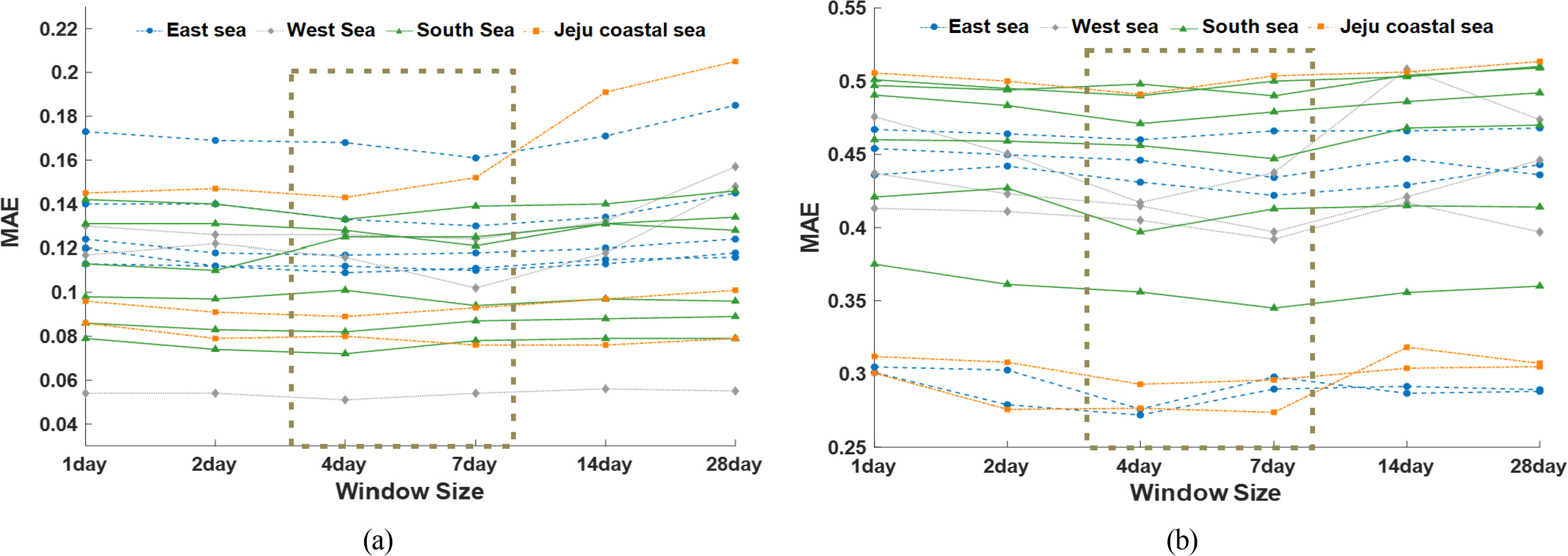
To present the wave prediction model by sea area, the observed data for each sea area were adjusted to the maximum interval of 30 min. Table 4 shows the MAE results of the wave prediction model by sea area. For the prediction of significant wave heights and significant wave periods, the GRU model achieved the optimal results at all the observation points except for the Korea Strait when the window size was either 4 d or 7 d (Figs. 4 (a) and (b)).
4.1.1 Significant wave height
For the significant wave height prediction results of the wave prediction model by sea area, the GRU model had the highest accuracy, followed by the RNN and LSTM models in order (Table 4). Fig. 4(a) shows the MAE results of the wave prediction model by sea area according to the window size, and the results at all the observation points had errors within 0.22 m of the observed values.
In the East Sea, the prediction of significant wave heights at Naksan Beach demonstrated a high prediction accuracy with an MAE ranging between 0.109 m and 0.116 m (Table 4, East Sea). Among these results, the MAE was 0.109 m when the model was trained for 4 d, showing a slight difference of 0.038 m from the MAE of the wave prediction model by observation point, which demonstrated the optimal value. The MAE value in the northeastern area of Ulleungdo was 0.161 m, which was the largest error among the observation points in the East Sea. Nevertheless, it only had a difference of 0.048 m from the MAE of the wave prediction model by observation point, indicating a good performance. The wave prediction model for the East Sea had accurate prediction results at all the observation points, with errors within 0.161 m of the observed values. It also showed an outstanding performance with differences within 0.048 m compared with the wave prediction model by observation point (Table 5, East Sea).
In the South Sea, the prediction results of the GRU model at Saengildo were closest to the observed values, with MAE values ranging between 0.072 m and 0.079 m (Table 4, South Sea). In particular, the MAE was 0.072 m when the model was trained for 4 d, and the difference from the results of the wave prediction model by observation point was 0.040 m. The eastern area of the South Sea had the largest error (0.133 m) among the observation points in the South Sea. However, it only had a slight difference of 0.039 m compared with the wave prediction model by observation point. Overall, the wave prediction model for the South Sea derived accurate prediction results, with errors within 0.133 from the observed results. Furthermore, it demonstrated an outstanding performance with differences within 0.047 m compared with the wave prediction model by observation point (Table 5, South Sea).
For the West Sea, the prediction results at Daecheon Beach were the most accurate among all the observation points in the West Sea, with errors ranging between 0.051 m and 0.056 m (Table 4, West Sea). Among these results, the MAE was 0.051 m when the window size was 4 d, showing a slight difference of 0.017 m from the MAE of the wave prediction model by observation point. Sangwangdeungdo had the highest error among all the observation points in the West Sea with an MAE of 0.124 m. However, this MAE has a difference of 0.025 m compared with that of the wave prediction model by observation point; hence, prediction results close to the observed results were derived. In the case of the wave prediction model for the West Sea, the MAE between the predicted results and the observed results was within 0.124 m at all the observation points. Furthermore, the differences were within 0.025 m compared with the wave prediction model by observation point, demonstrating the outstanding performance of the wave prediction model for the West Sea (Table 5, West Sea).
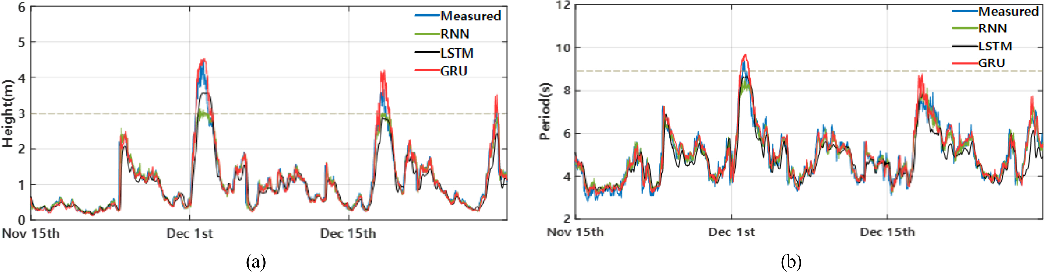
In the Jeju Coastal Sea, the Jeju Strait had the most accurate predictions with an MAE of 0.076 m when the window size was 7 d. The results showed a slight difference of 0.005 m compared with the wave prediction model by each observation point. On the other hand, the error was 0.143 m in the southern area of the Jeju Coastal Sea, and the prediction accuracy was relatively low. Moreover, the difference between these results and that of the wave prediction model by observation point was 0.0 m (Table 5, Jeju Coastal Sea). Fig. 5(a) shows a prediction graph of significant wave heights in the Jeju Strait in 2021. The prediction accuracy of the GRU model is higher than that of the other models on December 3 when the wave height is over 3 m. In addition, all the models demonstrated smaller errors when the wave height was 3 m or lower. Furthermore, the errors of the models excluding the GRU model increased gradually when the wave height was over 3 m (Table 6).
4.1.2 Significant wave period
Fig. 4(b) shows an MAE graph for the significant wave period of the wave prediction model by sea area according to the window size. The significant wave periods predicted by the wave prediction model by sea area exhibited errors within 0.55 s at all the observation points and had differences within 0.152 s compared with the prediction results of the wave prediction model by observation point. The accuracy of wave period predictions varied depending on the observation location; the prediction results were particularly accurate when the observation points were located in offshore seas rather than in nearshore seas. When waves move from an offshore sea toward a nearshore sea, phenomena, such as refraction and diffraction, can occur owing to a continental slope or the topography of the sea floor (Rhines and Bretherton, 1973). Owing to this process, waves in nearshore seas have variable characteristics compared with waves observed in offshore seas, which affects wave predictions.
In the East Sea, the MAEs at all the observation points were within 0.46 s, and the data measured at beaches ranged between 0.4 s and 0.5 s. The northeast and northwest areas of Ulleungdo, which are offshore seas, had the most accurate prediction results among the observation points in the East Sea, with the MAEs of 0.276 s and 0.272 s, respectively (Table 5, East Sea). Particularly, in the comparison between the wave prediction model by sea area and the wave prediction model by observation point, the differences at beaches were within 0.2 s. Furthermore, the wave prediction model by sea area provided more accurate results in Ulleungdo. Data by sea area are more diverse and consist of a larger amount of data than the data by observation point, and it is presumed that these aspects of the data have affected the learning of the model.
In the South Sea, the MAEs ranged between 0.447 s and 0.490 s at beaches besides Saengildo located in nearshore seas, the MAEs ranged between 0.345 s and 0.397 s in the eastern part of the South Sea and the Korea Strait, which are offshore seas. Of these results, the eastern part of the South Sea demonstrated an MAE of 0.345 s when the window size was 7 d, which was the most accurate among the results at the observation points in the South Sea. In particular, the results of the wave prediction model by sea area had very slight differences compared with those of the wave prediction model by observation point, ranging from 0.048 s to 0.134 s. Thus, the wave prediction model by sea area demonstrated an outstanding performance (Table 5, South Sea).
In the West Sea, the errors between the observed and predicted values at three observation points were not significant. Compared with the observed values, Sangwangdeungdo and Uido had the errors of 0.397 s and 0.417 s, respectively. In particular, the predicted results at Daecheon Beach had the highest accuracy among the observation points in the West Sea with an error of 0.392 s when the model was trained for 7 d. Moreover, the wave prediction model by sea area used in the West Sea demonstrated an outstanding performance with differences ranging between 0.066 s and 0.114 s compared with the results of the wave prediction model by observation point (Table 5, West Sea).
In the Jeju Coastal Sea, the optimal prediction result was observed in the southern area of the Jeju Coastal Sea with an MAE of 0.274 s when the window size was 7 d. The MAEs at the Jeju Strait and Jungmun Beach were 0.293 s and 0.491 s, respectively, when the model was trained for 4 d. Furthermore, the differences from the results of the wave prediction model by observation point were 0.056 s and 0.048 s at Jungmun Beach and the southern area of the Jeju Coastal Sea, respectively. On the other hand, the wave prediction model by sea area demonstrated a smaller error for the Jeju Strait, with a difference of 0.024 s (Table 5, Jeju Coastal Sea). Fig. 5(b) shows a graph of the prediction results of the significant wave period for the Jeju Strait in 2021. According to the graph, only the GRU model made predictions on December 3 when the wave period was 9 s or longer. Moreover, a comparison between Figs. 5 (a) and (b) shows that significant wave periods are 8 s or longer when significant wave heights are 3 m or higher, which shows that the wave height and the wave period have a proportional relationship.
Predictions made by the models used in this study were generally accurate, with errors within 0.57 m compared with the observed values. However, when the wave height was 3 m or higher or the wave period was 9 s or longer, only the GRU model demonstrated an outstanding prediction performance. Such prediction accuracy varies according to the structure and learning parameters of each model. If there are fewer learning parameters, the performance of learning complex patterns decreases, and the models have difficulty in learning long-term dependent data. Moreover, a problem occurs where previous information is lost over time. On the other hand, when there are several learning parameters, the computational efficiency decreases, and the risk of overfitting increases, which leads to a reduced accuracy. Therefore, appropriate learning parameters are necessary for accurate predictions. Among the three models that were executed under the same layer conditions, the GRU model compensated for the long-term dependency problems of RNNs. The GRU model also had an appropriate number of learning parameters with a simplified structure of an LSTM, and it demonstrated a high accuracy in wave predictions.
4.2 Optimal Wave Prediction Model by Each Location
The wave prediction model by observation point used the data measured at the actual measurement intervals of each observation point, considering the temporal continuity of the data. Table 4 shows that the GRU model demonstrated better prediction results than the RNN and LSTM models at all the observation points. Furthermore, the optimal values were determined for a window size of 4 or 7 d through Fig. 4. Therefore, the wave prediction model by observation point was executed by setting the window size that allows the wave prediction model by sea area to achieve the optimal value. Table 5 shows the MAE results at each observation point.
4.2.1 Significant wave height
The prediction results of significant wave height by observation point varied according to the actual measurement interval, and the prediction accuracy was relatively high when the actual measurement interval was within 5 min (Table 5). The data near the beaches in the East Sea were recorded every 5 min for the beaches in the East Sea and 30 min for Ulleungdo. Accurate prediction results were obtained for Gyeongpodae Beach, with an MAE of 0.068 m. Naksan Beach and Sokcho Beach had the MAE values of 0.071 m and 0.087 m, respectively, whereas the northeast and northwest areas of Ulleungdo had the MAE values of 0.113 m and 0.110 m, respectively (Table 5, East Sea).
In the South Sea, data were measured at intervals of 5 min or less at the beaches, whereas data were measured at intervals of 10 min at Saengildo. Moreover, data were measured at intervals of 30 min at all the other observation points. For the observation points located at the beaches, the MAE values ranged between 0.05 m and 0.075 m. In the case of the Korea Strait and the eastern area of the South Sea located in the offshore sea, the results were 0.093 m and 0.094 m, respectively. In particular, Saengildo had the best results among all the observation points, with an MAE of 0.032 m (Table 5, South Sea).
In the West Sea, data for each observation point were acquired differently depending on the location. Data were acquired at intervals of 5 min at Daecheon Beach and the MAE was 0.034 m, which is the most accurate prediction result among all the beaches. In the case of Sangwangdeungdo and Uido, data were measured at intervals of 10 min, and the MAE values were 0.099 m and 0.091 m, respectively (Table 5, West Sea).
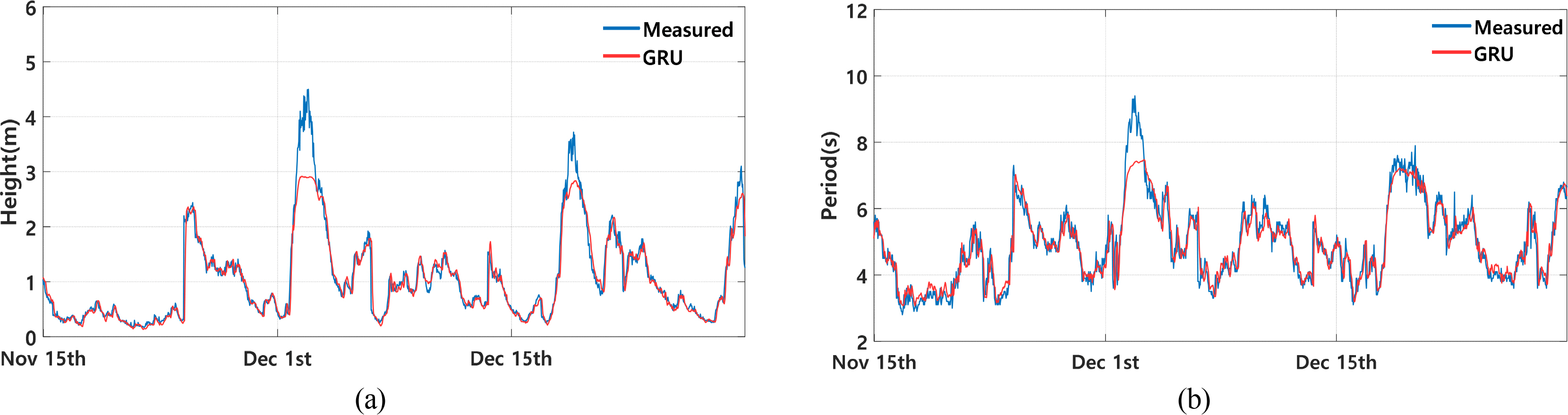
For the Jeju Coastal Sea, the data acquisition interval at Jungmun Beach was 5 min, and the MAE at this observation point was 0.074 m, which is the lowest error among the MAE values at all the observation points in the Jeju Coastal Sea. On the other hand, data were collected at intervals of 30 min at the Jeju Strait and the southern area of the Jeju Coastal Sea. The MAEs at these observation points were both 0.081 m (Table 5, Jeju Coastal Sea). Fig. 6(a) shows a graph of the prediction results of the significant wave height for the Jeju Strait in 2021. According to this graph, the prediction accuracy tends to decrease when the wave height is over 3 m. Table 6 shows the MAE values for each interval at the Jeju Strait, and the performance for each model can be analyzed based on these results. Notably, compared with the GRU wave prediction model by sea area, the differences between the two models were less than 0.067 m when the wave height was 3 m or less. Hence, the two models demonstrated relatively similar performances. However, the difference was 0.263 m when the wave height was between 3 m and 4 m, and the difference was 1.079 m when the wave height exceeded 4 m. Hence, as the wave height increased, the GRU wave prediction model by sea area produced more accurate predictions than the GRU wave prediction model by observation point.
4.2.2 Significant wave period
The errors for the prediction of significant wave periods were within 0.45 s at all the observation points, and the results were different depending on the observation location (Table 5). When waves move from an offshore sea toward a nearshore sea, they undergo transformations owing to various factors, such as the topography of the sea floor, refraction, and diffraction. Through this process, waves in nearshore seas have variable characteristics compared with relatively consistent waves observed in offshore seas, which affects wave predictions.
In the East Sea, the MAE values were derived to be approximately 0.3 s at all the observation points. The MAEs were 0.308 s for Gyeongpo Beach, 0.324 s for Naksan Beach, and 0.322 s for Sokcho Beach. In the case of Ulleungdo, which is located in the offshore sea, the northeast and northwest areas had the MAEs of 0.293 s and 0.299 s, respectively. Hence, they had smaller errors than the results for the beaches (Table 5, East Sea). In the South Sea, Haeundae Beach had an MAE of 0.356 s, Imrang Beach an MAE of 0.357 s, and Songjeong Beach an MAE of 0.363 s. Hence, MAE values of approximately 0.36 s were derived for the observation points at beaches. Moreover, Saengildo, which is located between islands, had the largest error, with an MAE of 0.416 s, among all the observation points in the South Sea. On the other hand, the Korea Strait and the eastern area of the South Sea, which are offshore seas, had the MAE values of 0.345 s and 0.297 s, respectively (Table 5, South Sea). In the West Sea, the wave prediction model by observation point exhibited errors ranging between 0.28 s and 0.33 s compared with the observed values. In particular, Daechon Beach had the largest error among all the observation points in the West Sea with an MAE of 0.326 s. Sangwangdeungdo and Uido had the MAE values of 0.283 s and 0.322 s, respectively (Table 5, West Sea). In the Jeju Coastal Sea, Jungmun Beach had an MAE of 0.435 s. On the other hand, the Jeju Strait and the southern area of the Jeju Coastal Sea, located in the offshore sea, had the MAE values of 0.298 s and 0.245 s, respectively (Table 5, Jeju Coastal Sea). Fig. 6 (b) shows a graph of the prediction results of the significant wave period for the Jeju Strait for the wave prediction model by observation point. According to this graph, the prediction accuracy of the GRU model decreases on December 2 if the wave period is 8 s or longer. Particularly, the difference between the MAE of the GRU wave prediction model by observation point and sea area is 0.133s when the wave period is less than 8 s. However, the difference is 0.387 s when the wave period is between 8 s and 9 s, and the difference is 1.480 s when the wave period exceeds 9 s. Hence, the prediction performance decreases as the wave period becomes longer.
In this study, various window sizes were applied to the RNN, LSTM, and GRU models to determine the optimized hyperparameters. In addition, this study presents a wave prediction model by sea area. To assess the performance, the optimized hyperparameters were applied to the prediction model by observation point, and the results were compared. The prediction model by sea area and the prediction model by observation point had slight differences in the significant wave height and significant wave period at all the observation points. The differences in significant wave height were within 0.062 m, and the differences in significant wave period were within 0.152 s. Hence, the prediction model by sea area demonstrated an outstanding prediction performance. The mean absolute percentage error (MAPE) was calculated to evaluate the relative magnitude of the prediction errors. The MAPE for significant wave height at all the observation points was within 18%, and the MAPE for significant wave period was within 10%. Hence, the prediction results similar to the observed values were derived. Moreover, to assess the significance of the research results, they were compared with the results of other studies. In a study by Hu (2021), waves in Lake Erie were predicted using ensemble techniques. In that study, the MAE of significant wave height was within 0.090 m (MAPE 17%), and the MAE of significant wave period was within 0.482 s (MAPE 13%). In a study by Minuzzi (2023), significant wave heights along the coast of Brazil were predicted using LSTM. In that study, the MAE was within 0.13 m (MAPE 7%), similar to the results of this study.
5. Conclusion
Marine operations, coastal management, and safety at sea are directly affected by waves. Particularly, accurate wave prediction is essential for marine development work in new locations. This paper proposed a wave prediction algorithm by sea area using data observed by oceanographic buoys. To build data by sea area, the data were integrated with maximum data intervals of 30 min, whereas data at each observation point were constructed with actual measurement intervals, considering the temporal continuity of the data. In addition, RNN, LSTM, and GRU, which are specialized for processing time-series data, were used as the algorithms. Furthermore, the optimized hyperparameters were determined by applying various window sizes. The results showed that GRU had the highest prediction accuracy when the window size was 4 or 7 d. In particular, it demonstrated excellent prediction accuracy for specific data with a wave height of over 3 m or a wave period of over 9 s. It is presumed that the simplified structure of the GRU and the appropriate number of learning parameters affected these results. Moreover, to assess the performance of the wave prediction model by sea area, the optimized hyperparameters were applied to the wave prediction model by observation point, and the results were compared. The comparison results showed that the wave prediction model by sea area and the wave prediction model by observation point, which considers the temporal continuity of the data, had slight differences in significant wave height and significant wave period at all the observation points. The differences were within 0.062 m for the significant wave height and 0.152 s for the significant wave period. Hence, the wave prediction model by sea area demonstrated an outstanding performance. Unlike previous studies, this study developed a method of predicting waves by building data for each sea area. This method can contribute to ensuring safety and enhancing work efficiency when conducting maritime and marine research at new locations. In addition, if the missing salinity, wave direction, and wave data can be acquired consistently, it is expected that waves will be predicted more accurately, and diverse waves will be predicted. Moreover, as data provided by the KHOA are used, it is expected that real-time wave predictions will be performed through online learning in the future.